
Some nice ML-libraries
I recently had a go at the Kaggle Acquire Valued Shoppers Challenge. This competition was a bit special in that the dataset was 22 GB, one of the biggest datasets they’ve had in a competition. While 22 GB may not quite qualify as big data, it’s certainly something that your average laptop will choke on when using standard methods. Ordinarily I’d reach for scikit-learn for these tasks, but in this case some of the methods in scikit-learn were a bit slow, and some other libraries had nice methods that scikit-learn didn’t have, so I decided to try out some other libraries. In this post I’ll give a brief look at some of the alternative machine learning libraries that I used during the competition.
In the Kaggle challenge, the intention was to predict whether a customer would become a “repeat buyer” of a product after trying the product. To give some examples of usage of the libraries I’m going through, I’ll use the features I created for the challenge, and predict probabilities of whether the customer was a “repeat buyer”. To follow the examples, you can download the features here and set up the training data for the examples like this:
import pandas as pd
train_data = pd.io.parsers.read_csv("./features/train/all_features.csv.gz", sep=" ", compression="gzip")
train_label = train_data['label']
del train_data['label']
del train_data['repeattrips']
test_data = pd.io.parsers.read_csv("./features/test/all_features.csv.gz", sep=" ", compression="gzip")
del test_data['label']
del test_data['repeattrips']
XGBoost
XGBoost (short for ‘extreme gradient boosting’) is a library solely devoted to, you guessed it, gradient boosting. Gradient boosting tends to be a frustrating affair, since it usually performs extremely well, but can also be very slow to train. Usually you would solve this by throwing several cores at the problem and use parallelization to speed it up, but neither scikit-learn or R’s implementation is parallellizable, and so there doesn’t seem to be much we can do. Fortunately there does exist alternative implementations that do support parallelization, and one of these is XGBoost.
XGBoost has a python API, so it is very easy to integrate into a python workflow. An advantage XGBoost has compared to scikit-learn, is that while scikit-learn only has support for gradient boosting with decision trees as “base learners”, XGBoost also has support for linear models as base learners. In our cross-validation tests, this gave us a nice improvement in predictions.
Another nice feature XGBoost has is that it will print out prediction error on a given test set for every 10 iterations over the training set, which allows you to monitor approximately when it starts to overfit. This can be used to tune how many rounds of training you want to do (in scikit-learn this is called n_estimators). On the other hand, XGBoost does not have support for feature-importances calculation, but they might implement this soon (see this issue).
In our example we first we create XGBoost train and test datasets, using the custom XGBoost DMatrix objects. We next set up our parameters: in the “param” dictionary, we set the max_depth of the decision trees, the learning rate of the boosting, here called eta, the objective of the learning (in our case logistic, since this is classification) and the number of threads we’d like to use. Since we had four cores when running this example, we set this to four threads. The number of rounds to do is set directly when we call the train method. We train via calling xgb.train(), and we can then call predict on our returned train object to get our predictions. Simple!
# import the xgboost library from wherever you built it
import sys
sys.path.append('/home/audun/xgboost-master/python/')
import xgboost as xgb

dtrain = xgb.DMatrix( train_data.values, label=train_label.values)
dtest = xgb.DMatrix(test_data.values)
param = {'bst:max_depth':3, 'bst:eta':0.1, 'silent':1, 'objective':'binary:logistic', 'nthread':4, 'eval_metric':'auc'}
num_round = 100
bst = xgb.train( param, dtrain, num_round )
pred_prob = bst.predict( dtest )
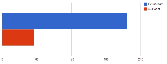
In our tests with four cores, it ran around four times as fast as scikit-learn’s GradientBoostingClassifier, which probably reflects the parallellization. With more cores, this would probably allow us to speed up the training even more. For some more detailed tutorials on how to use XGBoost, take a look at the documentation here.
A common problem with large data sets, is that usually you need to have the training data in memory to train on it. When the data set is big, this is obviously not going to work. A solution to this is so-called out-of-core algorithms, which commonly means only looking at one example from the training set at a time, in other words keeping the training data “out of core”. Scikit-learn has support for out-of-core/online learning via SGDClassifier, but in addition there also exists some other libraries that are pretty speedy:
Sofia-ml
Sofia-ml currently supports SVM, logistic regression or perceptron methods and uses some speedy fitting algorithms known as “Pegasos” (short for “primal estimatimated sub-gradient solver for SVM”). “Pegasos” has an advantage in that you do not need to define pesky parameters such as learning rate (see this article). Another nice feature in sofia-ml is that it supposedly also can optimize ROC area via selecting smart choices of samples when iterating over the dataset. “ROC area” is also known as AUC, which happened to be the score measure in our competition (and numerous other Kaggle competitions).
Using sofia-ml is pretty straightforward, but since it is a command-line tool, it easily seems a bit esoteric for those used to scikit-learn. Before we call the training, we have to write out the data to an input format called “SVMlight sparse data format” which originally comes from the library SMVlight, but has since been adopted by a number of other machine learning libraries. In our tests, what took the longest time was actually writing out the data, so we found it very helpful to use Mathieu Blondel’s library svmlight-loader, which does the writing out in C++. Note that there are also tools for handling SVMlight formats in scikit-learn, but they’re not quite as fast as this one.
There is no python wrapper for sofia-ml, but it’s quite easy to do everything from python:
from svmlight_loader import dump_svmlight_file
from subprocess import call
import numpy as np
from sklearn.preprocessing import StandardScaler

# normalize data
ss = StandardScaler()
train_data_norm = ss.fit_transform(train_data)
test_data_norm = ss.transform(test_data)

# change these filenames to reflect your system!
model_file = "/home/audun/data/sofml.model"
training_file = "/home/audun/data/train_data.dat"
test_file = "/home/audun/data/test_data.dat"
pred_file = "/home/audun/data/pred.csv"

# note that for sofia-ml (and vowpal wabbit), labels need to be {-1,1}, not {0,1}, so we change them
train_label.values[np.where(train_label == 0)] = -1

# export data
dump_svmlight_file(train_data_norm, train_label, training_file, zero_based=False)
dump_svmlight_file(test_data_norm, np.zeros((test_data.shape[0],)), test_file, zero_based=False)
We call the training and prediction with a python subprocess. In our first line, we specify via command-line parameters that the learner type is SVM fitted with stochastic gradient descent, use loop type ROC (to optimize for AUC), set prediction type “logistic” in order to get classifications, and do 200000 gradient descent updates. Many more possible command-line parameters are listed here. In the second line we create predictions on our test data from our model file, and we then read it in again via pandas. Note that in the case of logistic predictions, sofia-ml returns untransformed predictions, so we need to transform the predictions via the logistic transformation to get probabilities.
# train via subprocess call
call("~/sofia-ml/sofia-ml --learner_type sgd-svm --loop_type roc --prediction_type logistic --iterations 200000 --training_file "+training_file+" --model_out "+model_file, shell = True)

# create test data via subprocess call
call("~/sofia-ml/sofia-ml --model_in "+model_file+" --test_file "+test_file+" --results_file "+pred_file, shell = True)

# read in test data
pred_prob = pd.io.parsers.read_csv(pred_file, sep="\t", names=["pred","true"])['pred']
# do logistic transformation to get probabilities
pred_prob = 1./(1.+np.exp(-pred_prob))
In our tests, fitting using Sofia-ml was extremely speedy, around 3 seconds!
Vowpal Wabbit
This is probably the most well-known library to do fast out-of-core learning, and operates pretty similarly to sofia-ml. Vowpal Wabbit has support for doing SVM, logistic regression, linear regression and quantile regression via optimizing for respectively hinge loss, logit loss, squared loss and quantile loss. Since Vowpal Wabbit is written in C++, carefully optimized and has some tricks up it’s sleeve, it’s very fast and performs very competitively on a lot of tasks.
Vowpal Wabbit, like sofia-ml, is a command line program, and uses a slight modification of the SVMlight sparse data format for input. Since the differences between SVMlight and Vowpal Wabbits format were pretty small, we used the svmlight-loader library here as well, and modified the files to suit Vowpal Wabbit afterwards.
At the time of the competition, I didn’t find any python wrappers, but it seems there is now a python wrapper under development here. It’s not documented yet, so I’ll just use regular python methods to call Vowpal Wabbit in this example. First we have to write out training and test data:
training_file = "/home/audun/data/vw_trainset.csv"
training2_file = "/home/audun/data/vw_trainset2.csv"
test_file = "/home/audun/data/vw_testset.csv"
test2_file = "/home/audun/data/vw_testset2.csv"
pred_file = "/home/audun/data/pred.csv"
model_file = "/home/audun/data/vw_trainset_model.vw"

dump_svmlight_file(train_data, train_label, training_file, zero_based=False)
dump_svmlight_file(test_data, np.zeros((test_data.shape[0],)), test_file, zero_based=False)

# add specifics for vowpal wabbit format
import string
fi = open(training_file,"r")
of = open(training2_file,"w")
for lines in fi:
	li = lines.strip().split()
	of.write( li[0] )
	of.write(" | ")
	of.write( string.join(li[1:]," ") + "\n")
of.close()
fi.close()
fi = open(test_file,"r")
of = open(test2_file,"w")
for lines in fi:
	li = lines.strip().split()
	of.write( li[0] )
	of.write(" | ")
	of.write( string.join(li[1:]," ") + "\n")
of.close()
fi.close()
We then do a subprocess call to run Vowpal Wabbit from the command line. There are a lot of possible parameters to the command line, but all of them are listed here. The first line trains a model with logistic loss (i.e. for classification) on our training set, doing 40 passes over the data. The second line predicts data from our testset, based on our trained model, and writes the predictions out to a file.
# train
call("~/vowpalwabbit/vw "+training2_file+" -c -k --passes 40 -f "+model_file+" --loss_function logistic", shell=True)

# predict
call("~/vowpalwabbit/vw "+test2_file+" -t -i "+model_file+" -r "+pred_file, shell=True)
Next, we load the predictions from the output file. Note that like with sofia-ml the predictions need to be logistic transformed to get probabilities.
pred_prob = pd.io.parsers.read_csv(pred_file, names=["pred"])['pred']
pred_prob = 1./(1.+np.exp(-pred_prob))
Training is very fast, around 9 secs, even though the dataset is sizable. For a more in-depth tutorial on how to use Vowpal Wabbit take a look at the tutorial in their github repo.
So there you go, some nice, not-so-well-known machine learning libraries! In the competition overall, with the help of these libraries, I managed to end up in the top 10%, and together with my 4th place in the earlier loan default prediction competition, this earned me a “kaggle master” badge.
If you know of any other unknown but great libraries, let me know. And If you liked this blogpost, you should follow me on twitter!