In this blog post I'll describe some work I did a while ago in a consulting project together with Bengler. The work was a consultancy project for the national museum that was started in 2015 and the final result, VY, was made public in May last year. There were however some more experiments we tried during this project that I thought might be interesting to share.

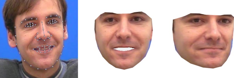
I was contacted by Bengler in 2014 regarding a potential project for Nasjonalmuseet. Nasjonalmuseet is Norways national gallery containing more than 30000 works of art, the most famous of them probably being Edvard Munchs' The Scream. The original proposal was to do something involving face recognition, since I'd released the face substitution demo not so long ago, but after some thought we decided to have a look at whether it would be possible to apply Deep Learning to the fine arts collection.

Visualization

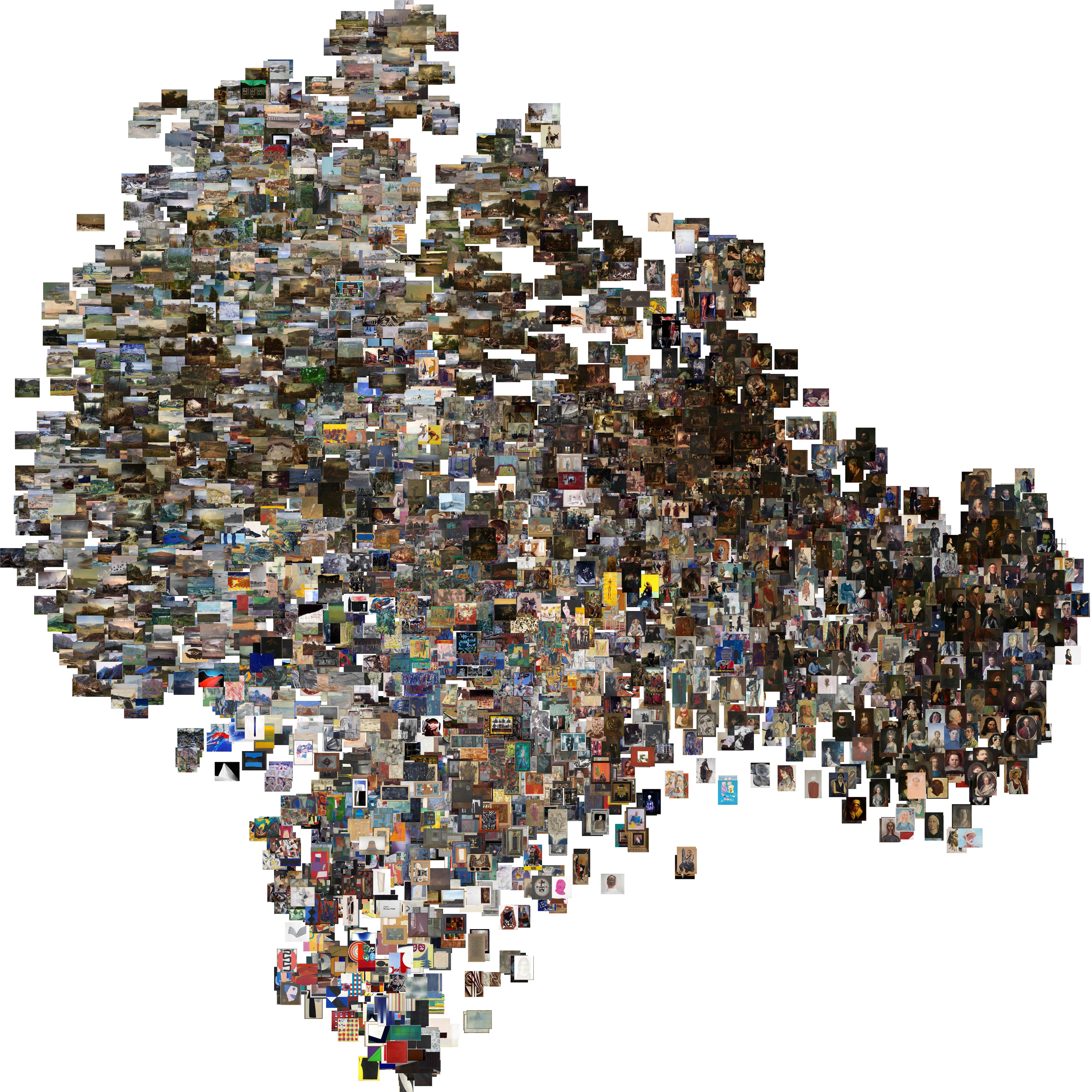
One of our first ideas was to try to visualize the collection in some way. Though the museum had webpages showing off parts of their collection, it was hard to get a complete overview of the entire collection as well as the many subjects found in the collection. t-SNE visualizations of deep learning features had worked well for another project of mine, so we decided to give this a try. At this point we had no idea whether this really would work for artworks as well, but as it turns out it did work really well.

In order to ensure that the embeddings became meaningful, we decided to train a deep learning classifier to classify artworks into art styles and motifs respectively. The models did not get super-high accuracy at that task, but that was not the main goal either. We simply wanted the features from the last layer of the trained classifier, which we used as input to a t-SNE model. As can be seen by the resulting t-SNE embedding below, this worked pretty well.

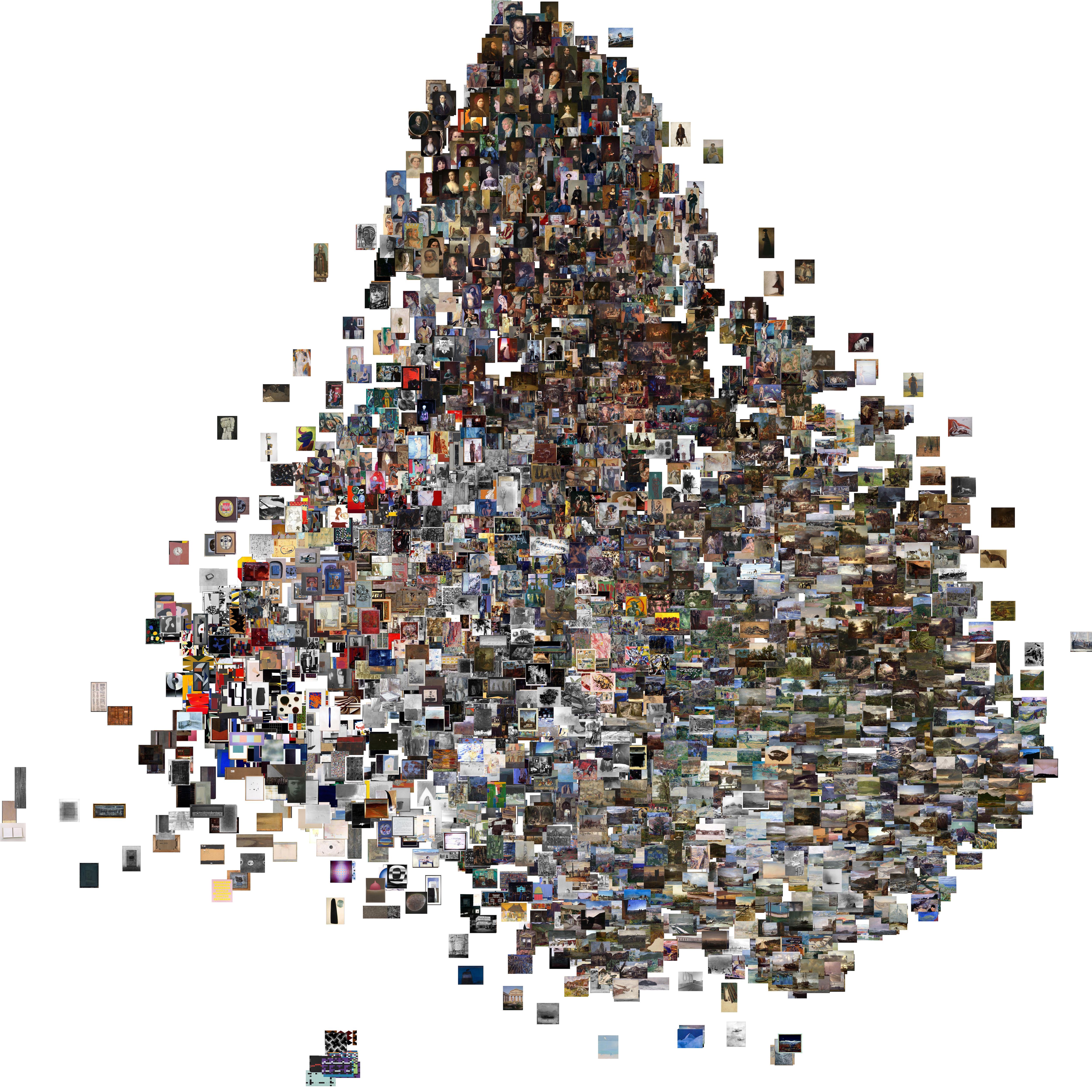
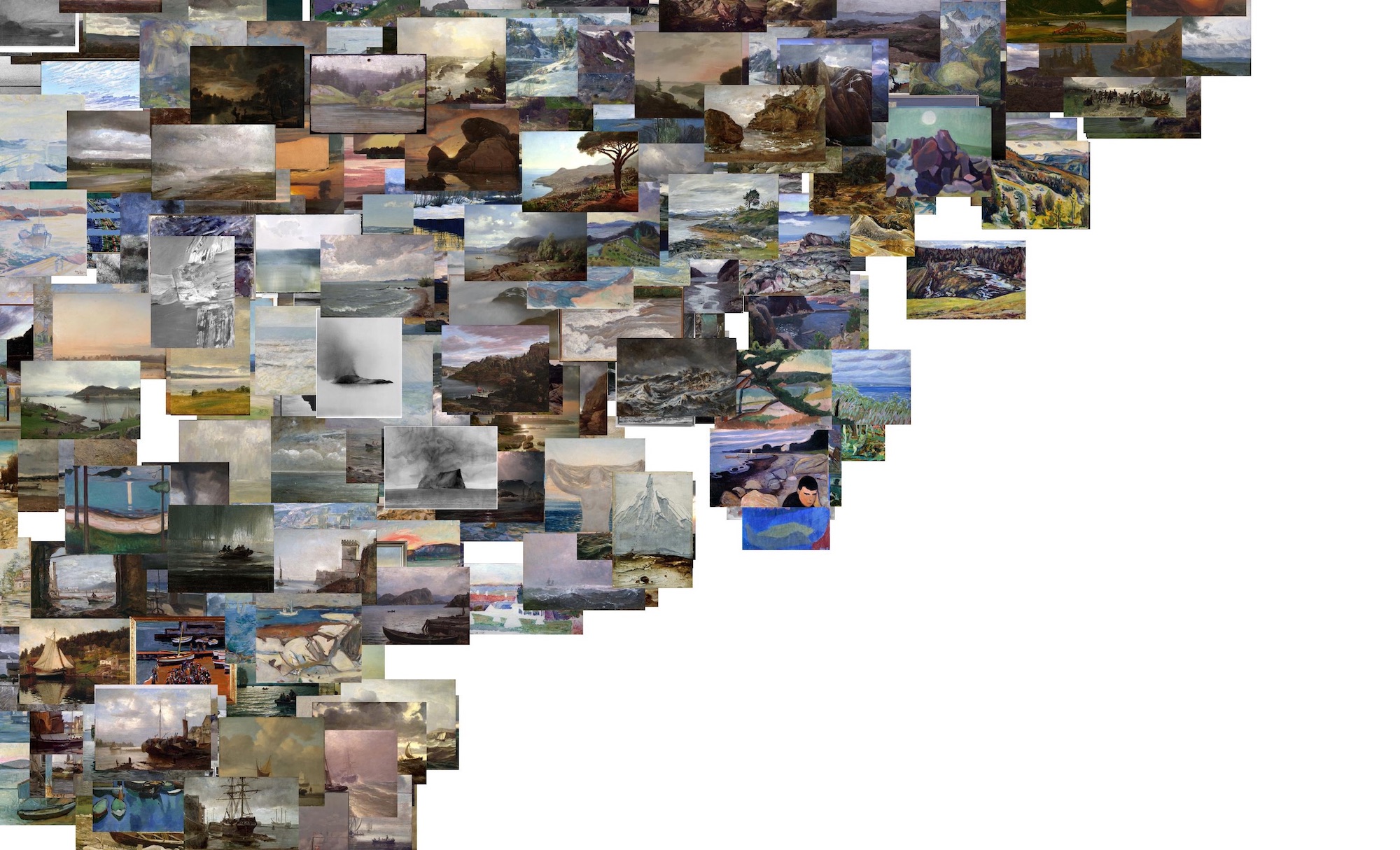
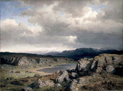
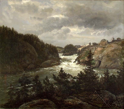
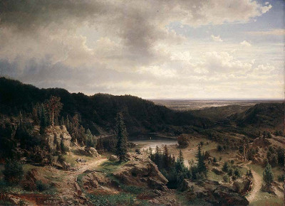
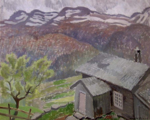
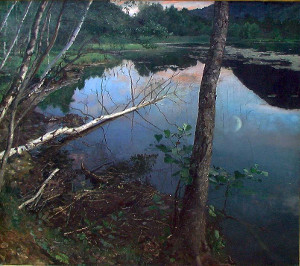
We got smooth transitions from nationalromantic paintings focusing on seas, through fjords, to forests.

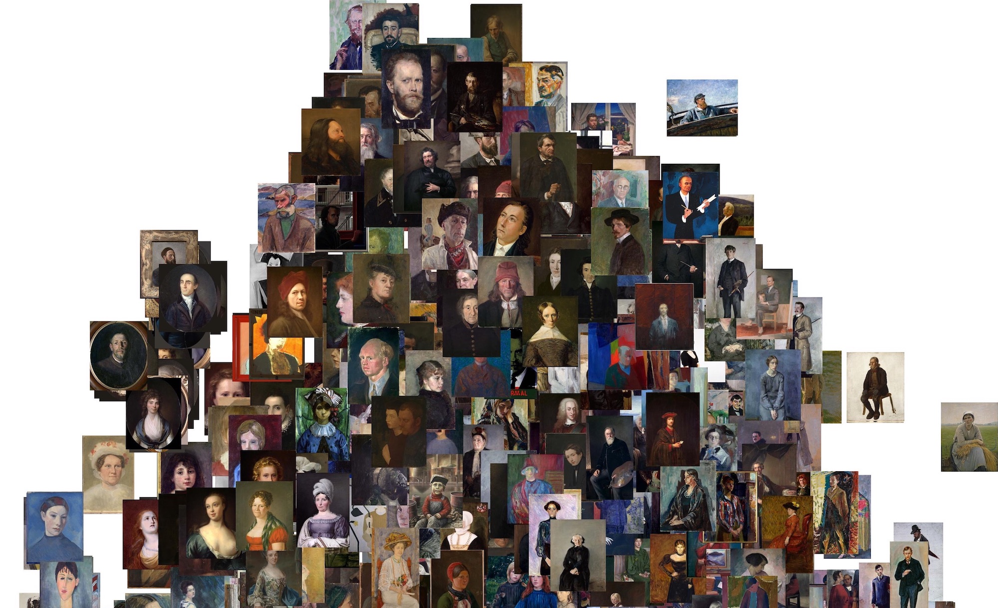
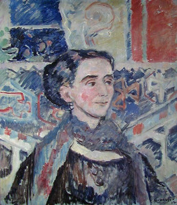
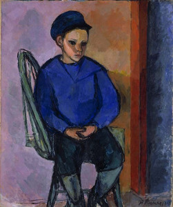
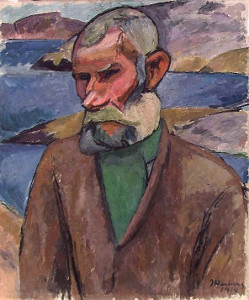
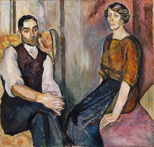
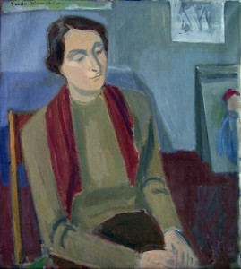
And from portraits one can clearly see clustering of women, bearded men, and full person portraits.

Visualizations were most interesting for paintings. Though they work just as well for drawings, it's harder to get a proper overview of the collection of the drawings, due to the reduced contrast of pencil drawings at small resolutions.

For the final public work we decided to try out parametric t-SNE, since we would have to make it possible for the t-SNE map to grow without having to retrain it for every addition to the collection. To our surprise, this seemed to give slightly better and more coherent t-SNE maps than the regular t-SNE method.

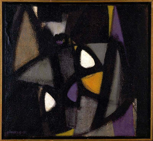
The features from our trained classifier can be used for more things than just visualization. We can also figure out what the typical works from a period looks like, by looking at works close to the mean embedding within a specific period. These works clearly show how typical norwegian painting gradually went from mainly nationalromantic landscape themes in mid 1800s, through to social realism at the turn of the century, and eventually abstraction in the fifties.

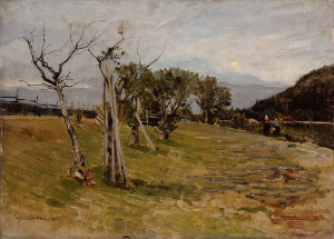
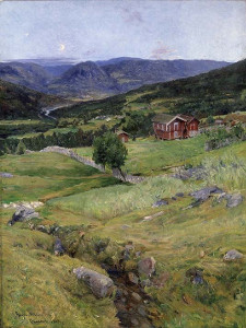
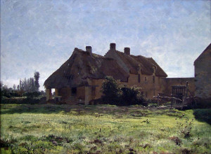
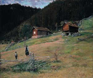
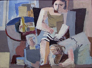
Similarly, we can also investigate if there are any stylistic outliers, by looking at works that are far from the mean embedding within each decade.

An interesting detail we noted is that outliers often signified trends that became commonplace a few decades later, such as the gradual shift to abstract painting.

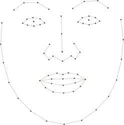
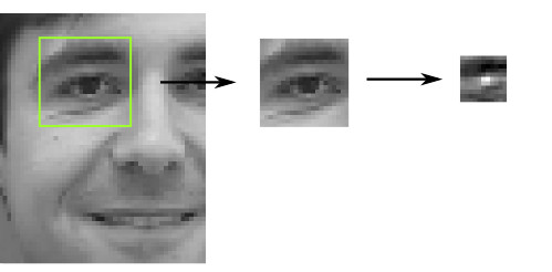
Faces in the collection

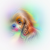
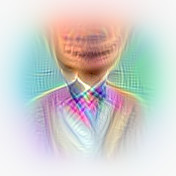
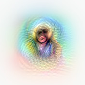
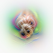
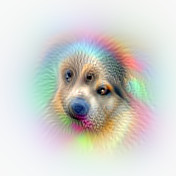
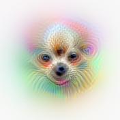
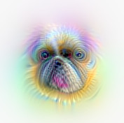
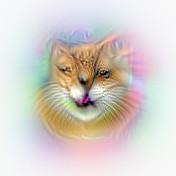
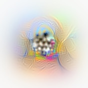
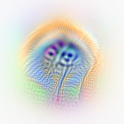
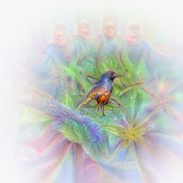
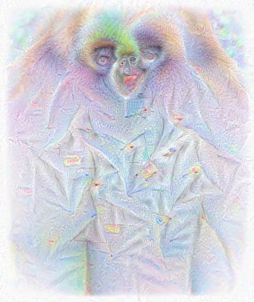
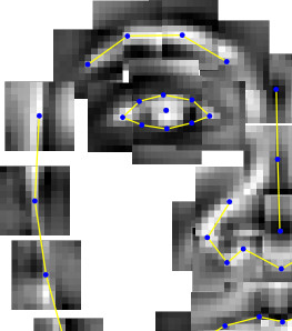
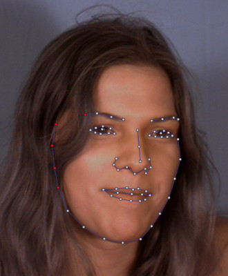
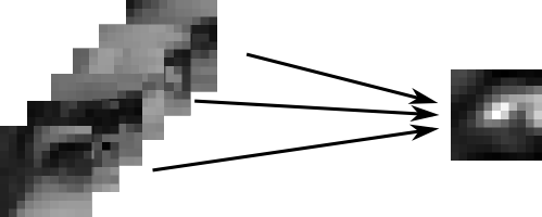
Since the original proposal involved doing something with faces in the collection, we also decided to have a look at applying similar visualization methods there. After detecting most faces in the collection and cropping them out, we tried out using a pretrained face-similarity embedding which we fed into a t-SNE model, but though the resulting embedding seemed to separate between male, bearded faces, and more feminine faces, the t-SNE visualizations didn't make quite as much sense as with the painting embeddings above. We suspected this might have to do with the difference between faces in paintings and photographies, so we even collected a dataset of painted fan-art of celebrities which we finetuned the face-similarity model on, but unfortunately it did not seem to have a significant effect on the quality of the visualization.

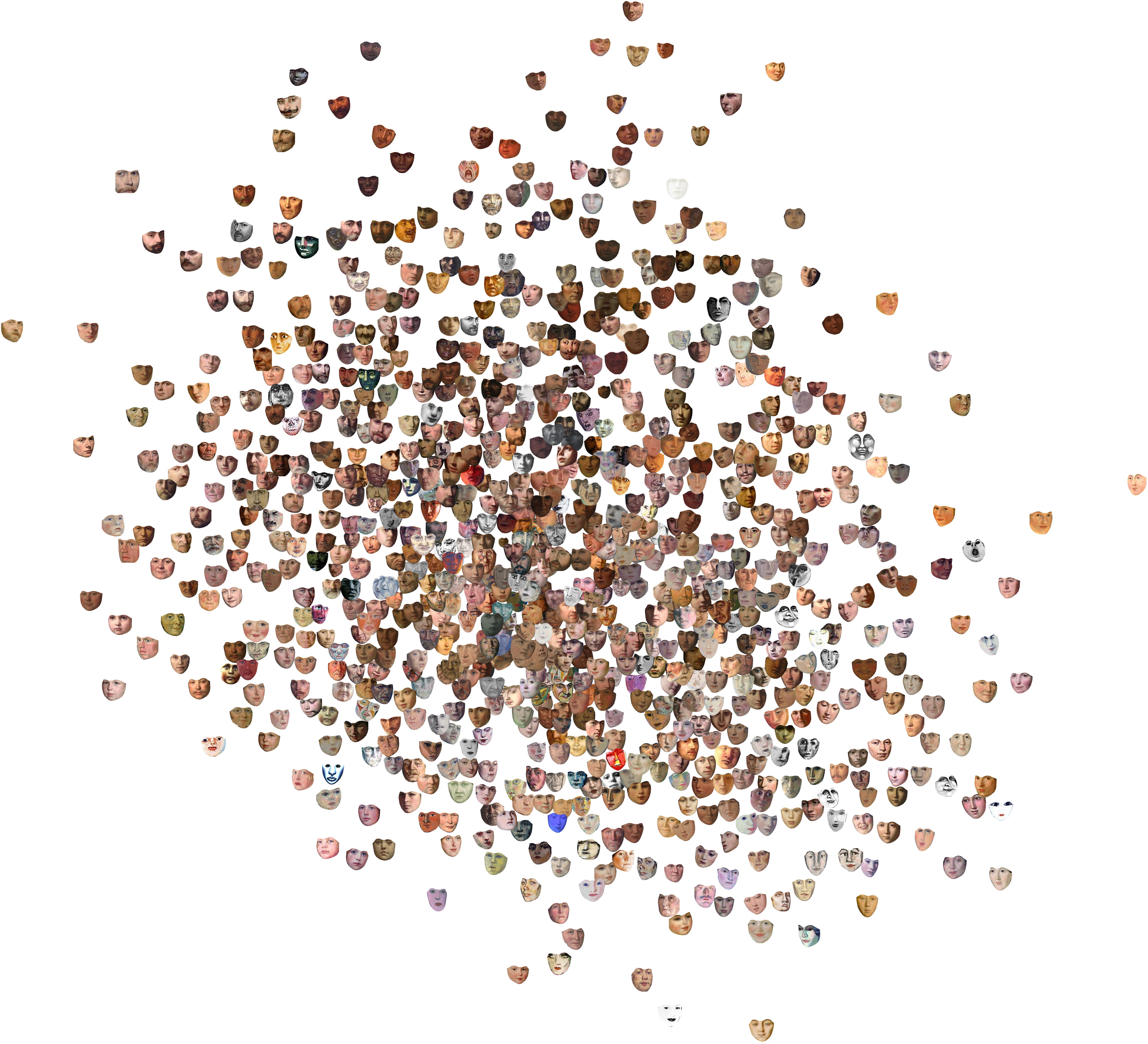
A follow-up idea we had was to make some kind of web app to allow visitors to find the faces in the collection most similar to their own, but due to time and budget constraints, we decided to scrap this idea. Fortunately, Google created just that a couple of months later, on a much larger collection of artworks.

Generating paintings

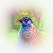
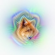
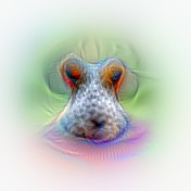
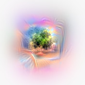
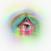
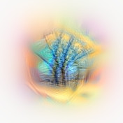
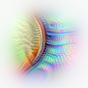
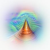
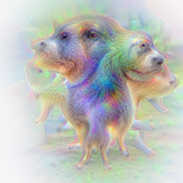
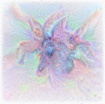
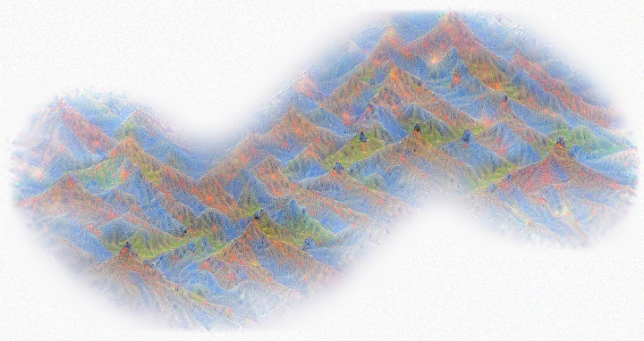
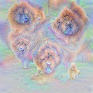
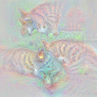
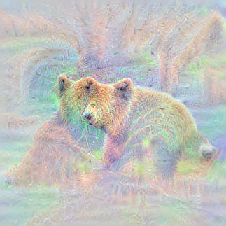
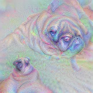
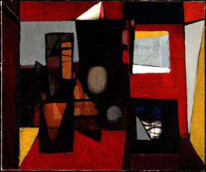
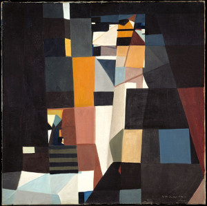
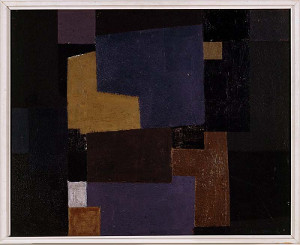
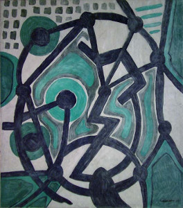
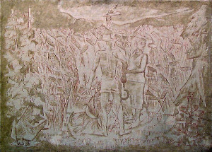
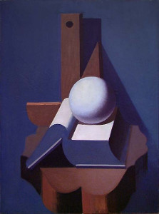
Of course, in 2016, sitting with a dataset of prime nationalromantic art, the temptation to train a Generative Adversarial Network on it was too strong. So naturally, we did just that. To train a DCGAN generating nationalromantic works, we first trained a GAN on a diverse set of styles of paintings from wikimedia, and then finetuned the model to a small augmented dataset of nationalromantic paintings. This is some of the results we got:

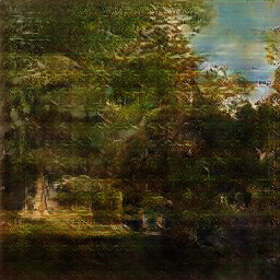
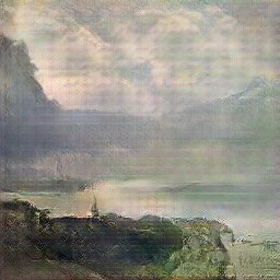
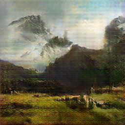
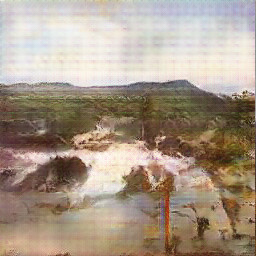
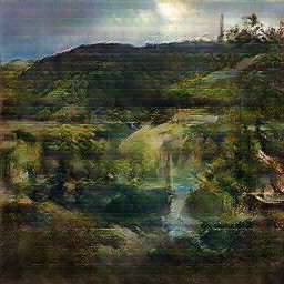
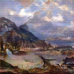
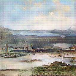
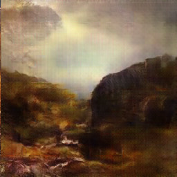
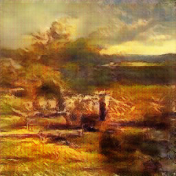
While they might not pass for authentic works by Tidemand & Gude, they do look like coherent, though vague nationalromantic paintings

We had no problem training a model (using DCGAN-tensorflow) to produce 256x256 paintings, though we quite often ran into the dreaded mode-collapse problem, which means all output converged to an abstract blob, so we'd have to start from scratch. We of course also tried to produce even larger 512x512 paintings, but this was more than our poor GPU RAM could handle. Efforts to scale up 256x256 images with superresolution also didn't work out well, since the superresolution mainly just sharpened artifacts in the image and added more noise.

Since we finished this project, there has been numerous improvements made to GAN models (one being Nvidia Researchs progressive growing GAN), which leads us to believe there is a huge potential to experiment more with GANs and art.

Conclusion

In finishing, I'd like to give a huge thanks to Bengler and the staff at the national museum, for their belief in the project and the free reins they gave us. Both during and after we worked on this project, we've seen similar projects, such as Googles Arts & Cultures Experiments, this, this and this. We believe there is lots of potential for fruitful collaboration between the fields of art and modern machine learning.

If you're interested in more info about what we did, also take a look at Benglers writeup of the project, as well as this blogpost on our experiments with training a model to classify paintings into iconclass classes.

If you enjoyed this post, you should follow me on twitter!

In a previous blogpost I showed how you could use gradient ascent, with some special tricks, to make a convolutional network visualize the classes it's learnt to classify. In this post I'll show that the same technique can also be used to "peek inside the network" by visualizing what the individual units in a layer detect. To give you an idea of the results, here's some highlights of visualizations of individual units from convolutional layer 5 in the VGG-S network:

From top left we can pretty clearly see the head of a cocker spaniel-type dog, the head of some kind of bird, the ears of a canine, and a seaside coastline. Not all unit vizualisations are as clearly defined as these, but most nevertheless give us some interesting insights into what the individual units detect.

Earlier methods for figuring out what the units detect (e.g. in Zeiler & Fergus) have been to find images which maximally activate the individual units. Here's an example of the images (sampled from numerous crops of 100 000 images in the imagenet validation dataset) which give maximal activations for a specific unit in layer 5 of VGG-S:

While this gives us an idea of what the unit is detecting, by visualizing the same unit we can see explicitly the details the unit is focusing on. Applying this technique to the same unit as above, we can see that the unit seems to focus on the characteristic pattern on the muzzle of the dog, seemingly ignoring most other details in the image.

We can use our visualization technique to get an overview of what all the different units in a typical layer detects. Here we've focused on convolutional layer 5 in VGG-S, which is the final convolutional layer in that specific network. Seemingly there are a large number of units that detect very specific features, such as (from top left below) forests/bushes in the background, buildings with pitched roofs, individual trees, clouds, collars, brass instruments, ship masts, bottle/jug tops, and seemingly the shoulders of people:

What is interesting to notice, is that the network doesn't seem to have learned detailed representations of faces. In e.g. the visualization featuring the collar, the face looks more like a spooky flesh-colored blob than a face. This might be an artifact of the visualization process, but it's not entirely unlikely that the network have either not found it necessary to learn the details, or not had the capacity to learn them.

There also are a surprisingly large number of units that detect dog-related features. I counted somewhere around 50, out of 512 units in the layer in total, which means a surprising 10% of the network may be dedicated solely to dogs. Here's a small sample of these:

On the other hand I could only find a single unit that clearly detected cat features (!):

Some of the units are more general shape detectors, detecting edges, circles, corners, cones or similar:

and some seem to detect textures, such as these detecting leopard fur and wood grain:

Not all of the unit visualizations are so easy to interpret, such as these:

However, if we find images that maximally activate these units, we can see that they detect respectively grids and more abstract features such as out-of-focus backgrounds, and shallow-focus/macro images.

Overall, this visualization of the units give us useful insight into what the units in VGG-S detect. However, VGG-S is a relatively shallow network by todays standards, with only 5 convolutional layers. What about visualizing units in deeper networks, such as VGG-16 or GoogLeNet? Unfortunately, this doesn't seem to work as well, though it gives us some interesting results. Here for instance, is a visualization of some units in convolutional layer 4c from GoogLeNet:

You might recognize some of these as the "puppyslugs" from DeepDream. While these visualization are more detailed than the ones we get from VGG-S, they also have a tendency to look more psychedelic and unreal. It is not completely clear why this happens, but it seems like the center of the visualization generally seems to be a good representation of what the unit detects, while the edges gives us lots of random details.

Similarly for VGG-16, the visualizations we get are much harder to interpret, though we can see in some of these that the unit seems to detect respectively some kind of dog, a theater and a brass instrument (with players as blobs).

A hypothetical reason that these visualizations doesn't work as well for deeper networks, has to do with the nature of the convolutional networks. What each convolutional layer tries to do is to be able to detect specific features, without being sensitive to irrelevant variations such as pose, lighting, partial obstruction etc. In this sense, each convolutional layer "compresses" information and throws away irrelevant details such as pose etc. This works great when doing detection, which is what the network is actually meant to do. However, when we try to run the network in reverse and generate feasible images, for each layer we have to "guess" the irrelevant structural details that have been thrown away, and as the choices made in one layer might not be coordinated with other layers, this in effect introduces some amount of "structural noise" for each layer we have to run in reverse. This might be a minor issue for networks with few layers, such as VGG-S, but as we introduce more and more layers, the cumulative "structural noise" might simply overpower the generated structure in the image, and make the image look much less like what we would recognize as e.g. a dog, and more like what we recognize as the "puppyslugs" seen in DeepDream.

More investigations might have to be done to tell whether this is actually the reason that visualization fails for deeper networks, but I wouldn't be surprised if this is part of the reason. Below I briefly describe the technical details of how I made these visualizations.

Technical details

To visualize the features, I'm using pretty much the same technique I described earlier in this blogpost, starting from a randomly initialized image, and doing gradient ascent on the image with regards to the activation of a specific unit. We also use blurring between gradient descent iterations (which is equivalent to regularization via a smoothness prior), and gradually reduce the "width" of the blur during gradient descent in order to get natural-looking images. Since units in intermediate layers actually output a grid of activations over the entire image, we choose to optimize a single point in this grid, which gives us a feature visualization corresponding to the units receptive field.

Another trick I also used, was to modify the network to use leaky ReLUs instead of regular ReLUs, since otherwise the gradient will usually be zero when we start from a blank image, thus hindering initial gradient ascent. Since this modification doesn't seem to have significant effect on the predictions of the network, we can assume it doesn't have a major impact on the feature visualizations.

I've released the code I used to make these visualizations, so take a look if you want to know more details.

Similar work

There has been similar work on visualizing convolutional networks by e.g. Zeiler and Fergus and lately by Yosinski, Nugyen et al. In a recent work by Nguyen, they manage to visualize features very well, based on a technique they called "mean-image initialization". Since I started writing this blog post, they've also published a new paper using Generative Adversarial Networks as priors for the visualizations, which lead to far far better visualizations than the ones I've showed above. If you are interested, do take a look at their paper or the code they've released!

If you enjoyed this post, you should follow me on twitter!

There’s nothing constraining us to generate image examples of one class at a time. Let’s see what happens if we try to generate two class visualizations close to each other, such as for instance a gorilla and a french horn

Well, it kind of looks like a gorilla playing the french horn. Or let’s try dressing up a gibbon via “mixing” the gibbon class with some of the clothing classes:

Or what about making some scenic nature drawings, such as some foxes underneath an erupting volcano:

Or a ballpoint pen drawing a castle:

These mixes of classes kind of work out, though it should be noted that these are the best selections from a number of mixes I tried. It’s also tempting to create mixes of animal classes to generate some new kind of monster breeds, but most of the time this doesn’t work so well. Here’s some I tried though, a mix of a scotch terrier and a tarantula, and a mix of a bee and a gibbon:

Another fun thing we can do when generatinge images is to do the gradient ascent randomly along paths instead of on a single point. This of course takes a bit longer time, but it allows us to “draw” with the output, such as for instance drawing a mountain range of alps:

or a line of jellyfish:

or a circle of junco birds:

If we try to fill a larger region with visualizations of a class, we can also apply clipping masks, i.e. forcing the pixels to zero in some pattern during gradient ascent. So we can for instance use letters as clipping masks and try to create the alphabet with animals:

Alright, that’s enough abuse of our deep neural network for today. I’ve just scratched the surface here, but there are several fun ways to use deep neural networks for creative visual work with a bit of experimentation (and lots of patience). I’m going to put the ipython notebooks I used to make these examples in the deepdraw repository as soon as I’ve cleaned up the code, so stay tuned via twitter.

Recently Google published a post describing how they managed to use deep neural networks to generate class visualizations and modify images through the so called “inceptionism” method. They later published the code to modify images via the inceptionism method yourself, however, they didn’t publish code to generate the class visualizations they show in the same post.

While I never figured out exactly how Google generated their class visualizations, after butchering the deepdream code and this ipython notebook from Kyle McDonald, I managed to coach GoogLeNet into drawing these:

It should be mentioned that all of these images are generated completely from noise, so all information is from the deep neural network, see an example of the gradual generation process below:

In this post I’ll describe a bit more details on how I generated these images from GoogLeNet, but for those eager to try this out yourself, jump over to github where I’ve published ipython notebooks to do this yourself. For more examples of generated images, see some highlights here, or visualization of all 1000 imagenet classes here.

Aside from the fact that our network seems to be drawing with rainbow crayons, it’s remarkable to see how detailed the images are. They’re far from perfect representations of the objects, but they give us valuable insight into what information the network thinks is essential for an object, and what isn’t. For instance, the tabby cats seem to lack faces while the dalmatians are mostly dots. Presumably this doesn’t mean that the network hasn’t learned the rest of the details of these objects, but simply that the rest of the details are not very discriminate characteristics of that class, so they’re ignored when generating the image.

As google also noted in their post, there are often also details that actually aren’t part of the object. For instance, in this visualization of the “Saxophone” class there’s a vague saxophone player holding the instrument:

This is presumably because most of the example images used for training had a saxophone player in them, so the network sees them as relevant parts of the object.

In the next part I’ll go a bit into details on how the gradient ascent is done. Note : this is for specially interested, with some knowledge of deep neural networks being necessary.

Generating class visualizations with GoogLeNet

In order to make a deep neural network generate images, we use a simple trick. Instead of using backpropagation to optimize the weights, which we do during training, we keep the weights fixed and instead optimize the input pixels. However, trying to use unconstrained gradient ascent to get a feasible class visualization works poorly, giving us images such as the one below.

The reason for this is that our unconstrained gradient ascent quickly runs into local maximums that are hard to get out of, with high frequency and low frequency information competing and creating noise. To get around this, we can choose to just optimize the low-frequency information first, which will give us the general structure of the image, and then gradually introduce high-frequency details as we continue gradient ascent, in effect “washing out” an image. Doing this in a slow way, we manage to ensure that optimization converges with a feasible image. There are two possible routes for doing this:

• applying gaussian blur to the image after we’ve applied the gradient step, starting with a large sigma and slowly decreasing it as we iterate
• applying gaussian blur to the gradient, starting with a large sigma and slowly decreasing it as we iterate (note that in this case we also have to use L2-regularization of the pixels to gradually decrease irrelevant noise from previous iterations)

I’ve had best results with the former approach, which is the approach I used to generate the images above, but it might be that someone might get better results with blurring the gradient via messing about with the parameters some more.

While this approach works okayish for relatively shallow networks like Alexnet, a problem you’ll quickly run into when doing this with GoogLeNet, is that as you gradually reduce the amount of blurring applied, the image gets saturated with high-frequency noise like this:

The reason for this problem is a bit uncertain, but might have to do with the depth of the network. In the original paper describing the GoogLeNet architecture, the authors mention that since the network is very deep, with 22 layers, they had to add two auxiliary classifiers at earlier points in the network to efficiently propagate gradients from the loss all the way back to the first layers. These classifiers, which were only used during training, ensured proper gradient flow and made sure that early layers were getting trained as well.

In our case, the pixels of the image are even further ahead in the network than first layer, so it might not seem so surprising that we have some problems with gradients and recovering a feasible image. Exactly why this affects high-frequency information more than low-frequency information is a bit hard to understand, but it might have to do with gradients for high-frequency information being more sensitive and unstable, due to larger weights for high-frequency information, as mentioned by Yosinski in the appendix to this paper.

While the auxiliary classifiers in GoogleNet are only used during training, there’s nothing stopping us from using them for generating images. Doing gradient ascent on the first auxiliary classifier, we get this:

while the second auxiliary classifier gives us this:

As can be seen, the first classifier easily manages to generate an image without high-frequency noise , probably because it’s “closer” to the early layers. However, it does not retain the overall structure of the object, and peppers the image with unnecessary details. The reason for the lack of structure is that the deeper a network is, the more structure the network is able to learn. Since the first classifier is so early in the network, it has not yet learned all of the structures deeper layers has. We can similarly see that the second classifier has learned some more structure, but has slightly more problems with high-frequency noise (though not as bad as the final classifier).

So, is there any way to combine the gradients from these classifiers in order to ensure both structure and high-frequency information is retained? Doing gradient ascent on all three classifiers at the same time unfortunately does not help us much, as we get both poor structure and noisy high-frequency information. Instead, what we can do is to first do gradient ascent from the final classifier, as far as we can before we run into noise, then switch to doing gradient ascent from the second classifier for a while to “fill in” details, then finally switching to doing gradient ascent from the first classifier to get the final fine-grained details.

Another trick we used, both to get larger images and better details, was to scale up the image at certain intervals, similar to the “octaves” used in the deepdream code. Since the input image the network optimizes is restricted to 224x224 pixels, we randomly crop a part of the scaled up image to optimize at each step. Altogether, this gives us this result:

Though this approach gives us nicely detailed images, note that both the scaling and the auxiliary classifiers tend to degrade the overall structure of the image, and particularly larger objects often tend to be “torn apart”, such as this dog gradually turning into multiple dogs.

Since the network actually seems to be capable of creating more coherent objects, it’s possible that we could generate better images with clever priors and proper learning rates, though I didn’t have any luck with it so far. Purely hypothetically, deep networks with better gradient flow might also be able to recover more detailed and structured images. I’ve been curious to see if networks with batch normalization or Parametric ReLUs are better at generating images since they seem to have better gradient flow, so if anyone has a pretrained caffe model with PReLUs or batch normalization, let me know!

Another detail that’s worthy to note is that we did not optimize directly the loss layer, as the softmax denominator makes the gradient ascent put too much weight on reducing other class probabilities. Instead, we optimize the next to last layer, where we can make the gradient ascent focus exclusively on optimizing a likely image from our class.

As a final side note it’s very interesting to compare the images AlexNet and GoogLeNet generate. While the comparison might not be entirely representative, it certainly looks like Googlenet has learned a lot more details and structure than AlexNet.

Now go ahead and try it yourself! If you figure out other tricks or better choices of parameters for the gradient ascent (there almost certainly are), or just create some cool visualizations, let me know via twitter!

A big hat tip to google and their original deepdream code, as well as Kyle McDonald, which had the original idea of gradually reducing sigma of gaussian blurring to “wash out” the image, and kindly shared his code.

Sequential analysis tests, such as the sequential GLR test I wrote about in my previous post, allows us to save time by stopping the test early when it’s possible. However, the fact that the test can stop early has some subtle consequences for the estimates we make after the test is done. Let’s take a look at the average maximum likelihood estimate when applied to the “comparison of proportions” sequential GLR test:

It seems like the average estimate is slightly off - to get a better view, let’s take a look at just the bias, i.e. the average ML estimate minus the true difference :

The estimates are (almost imperceptably) biased inwards when the true difference is close to zero, biased outwards when the difference between proportions are relatively large, and then unbiased again at the extreme ends. This is quite unlike fixed sample-size tests, which have no such bias at all. The reason for this difference is that there is an interaction between the stopping time and the estimate - sequential tests stop early when our samples are more extreme than some threshold, which means that the final estimates we get more often than not will be more extreme than what is true.

This might become a bit more intuitive if we take a look at a typical sample path for the MLE and the approximate thresholds for stopping the test in terms of the MLE. In this case the true difference is 0.2, and we do a two-sided sequential GLR test with α-level 0.05, β-level 0.10 and indifference region of size 0.1 :

As we collect data, the ML estimates jump quite a bit around before converging towards the true difference. As it jumps around, it's likely to cross the threshold at a higher point (as seen happening here after around 70 samples) and thus stop the test at this point. Similarly, when the true difference is close to zero, it will usually stop at values slightly closer to zero than the actual difference. What about the vanishing bias at the extremes? This is because at the most extreme values, the test will almost invariably stop at only a handful of samples, and thus the interaction between the stopping time and the estimate practically disappears.

So what can we do about this problem? Unfortunately, there is not an uniformly best estimator we can use as a replacement for the MLE. Some of the estimators suggested to fix the bias have much larger mean squared error than the MLE due to having larger variance. However, a simple and commonly used correction (and what we use in the sequential A/B-testing library SeGLiR), is the Whitehead bias-adjusted estimate. The Whitehead bias-adjusted estimate is based on the fact that we know that:

E(\hat{\theta}) = \theta + b(\theta)

where theta is the true difference, theta_hat is our estimate of the difference, and b(theta) is the bias of our test at theta. Given an estimate theta_hat, we can then find an approximately bias-adjusted estimate by solving for theta_sim so that:

\tilde{\theta} + b(\tilde{\theta}) = \hat{\theta}

This can be found by simple simulation and some optimization. Note that there are also other alternative estimators, such as the conditional MLE, but since the brute-force simulation approach to this would take much more time than the Whitehead bias-adjustment, it's not something I've implemented in SeGLiR currently.

One important thing to note is that the bias problem is not specific to the sequential GLR test or even sequential frequentist tests. In fact any test with a stopping rule that depends on the parameter we estimate, such as Thompson sampling with a stopping rule (as used by google analytics) will have the same problem. John Kruschke discusses this in the context of bayesian analysis in this blog post.

Precision and Confidence intervals

So, given that we've bias-corrected the estimates, how precise are the estimates we get? Unfortunately, estimates from sequential analysis tests often are less precise than the fixed sample-size test. This is not so surprising, since the tests often stop earlier, and we thus have less data to base the estimates on. To see this for yourself, take a look at the estimates given in this demo.

For this reason, it is natural to ask for confidence intervals to bound the estimates in sequential analysis tests. Classical fixed sample-size tests use the normal approximation to create confidence intervals for the estimate. This is usually not possible with sequential analysis tests, since the distribution of the test statistics under a stopping rule are very complex and usually impossible to approximate by common distributions. Instead we can resort to bootstrap confidence intervals, which are simple to simulate. These are unfortunately also sensitive to the bias issues above, so the best option is to use a bias-adjusted confidence interval^[1]. Note that since sequential tests stop early and we often have fewer samples, the confidence intervals will usually be wider than for the fixed sample-size test.

[1] see Davison & Hinkley : Bootstrap Methods and their applications, chap. 5.3 for details

P-values

As a little aside, what about p-values, the statistic everyone loves to hate?

When doing classical hypothesis tests, p-values are usually used to describe the significance of the result we find. This is not quite as good an idea in sequential tests as in fixed sample-size tests. The reason for this is that the p-value is not uniquely defined in sequential tests. The p-value is defined as the probability that we get a result as extreme or more extreme than the one we see, given that the null-hypothesis is true. In fixed sample-size tests, a more extreme result is simply a result where the test statistic is well, more extreme. However, in the sequential setting, we also have the variable of when the test was stopped. So is a more “extreme result” then a test that stops earlier? Or a test that stops later, but with a more “extreme” test-statistic? There is no definite answer to this. In the statistical literature there are several different ways to “order” the outcomes and thus define what is more “extreme”, but unfortunately there is no consensus on which “ordering” is the best, which makes p-values in sequential analysis a somewhat ambiguous statistic.

Nevertheless, in SeGLiR we've implemented a p-value via simple simulation, where we assume that a more “extreme result” is any result where the test statistic is more extreme than our result, regardless of when the test was stopped. This is what is called a Likelihood Ratio-ordering and is the ordering suggested by Cook & DeMets in their book referenced below.

As we've seen in this post, estimation in sequential tests is a bit more tricky than in fixed sample-size tests. Because sequential tests use much less samples, estimates may be more imprecise, and because of the interaction with the stopping rule they tend to be biased, though there are ways to mitigate the worst effects of this. In an upcoming post, I'm planning to compare sequential analysis tests with other variants of A/B-tests such as multi-armed bandits, and give a little guide on when to choose which test. If you're interested, follow me on twitter for updates.

References

If you're interested in more details on estimation in sequential tests, here are some recommended books that cover this subject. While these are mostly about group sequential tests, the solutions are the same as in the case with fully sequential tests (which is what I've described in my posts).

• C. Jennison & B. Turnbull : Group Sequential Methods with Applications to Clinical Trials, CRC Press 1999
• T. Cook & D. DeMets : Introduction to Statistical Methods for Clinical Trials, Chapman & Hall/CRC Press 2007

The Sequential Generalized Likelihood Ratio test (or sequential GLR test for short) is a test that is surprisingly little known outside of statistical clinical research. Unlike classical fixed sample-size tests, where significance is only checked after all samples have been collected, this test will continously check for significance at every new sample and stop the test as soon as a significant result is detected, while still guaranteeing the same type-1 and type-2 errors as the fixed-samplesize test. This means the test could be stopped as early as after a handful of samples if there is a strong effect present.

Despite this very nice property, I couldn’t find any public implementation of this test, so I’ve created a node.js implementation of this test, SeGLiR, which can easily be used in web application A/B testing. I’ll give a brief example of usage below, but to give you some idea about the potential savings, I’ll first show you a comparison of the needed samplesize for a fixed samplesize test versus the sequential GLR test.

The test I’ll compare is a comparison of proportions test, which is commonly used in A/B-testing to compare conversion rates. We compare the tests at the same levels, α-level 0.05 and β-level 0.10, and say that we want to detect a difference between proportions larger than 0.01 (in sequential analysis this is usually called an “indifference region” of size 0.01). Note that the expected samplesize for the sequential GLR test vary depending on the true proportions p₁ and p₂, so we compare the samplesize at different true proportions. We’ll first look at the case where the expected samplesize for the sequential GLR test is worst, when the proportions are closest to 0.5.

As you can see, the expected samplesize of the sequential GLR test is much smaller for almost any value of the true difference. The test will stop especially early when there is a large difference between the proportions, so if there is a significant advantage of choosing one of the alternatives, this can be acted upon as early as possible. Let’s take a closer look at the expected samplesize when the differences between the true proportions are small.

The only case where the sample size for the sequential GLR test can be expected to be larger, is when the true difference between p₁ and p₂ is just below 0.01, i.e. the smallest difference we were interested in detecting. However, this is just when the proportions are close to 0.5. What about when p₁ and p₂ are farther from 0.5?

Actually, as the true p₁ and p₂ get closer to either 0 or 1, the expected samplesize will always be smaller than the fixed samplesize test. Since this is the expected samplesize, to be sure that the test doesn’t often require a much higher samplesize, let’s also take a look at the more extreme outcomes, for instance the 5th and 95th percentiles (with p₁ and p₂ close to 0.5 as earlier):

For most of the true differences the samplesize is still lower than the fixed-samplesize test, except for differences below 0.015. A good next question might be if there is a bound to the amount of samples we may have to collect? Actually, there exists a worst-case samplesize for the test, meaning that the test will always conclude before this point. In the example above, the worst-case samplesize, though extremely rare, is at 161103 samples. Note that there is a tradeoff between this worst-case samplesize and the size of the indifference region, which means that a smaller indifference region will lead to a larger worst-case samplesize, and a larger indifference region will lead to a smaller worst-case samplesize.

Given the very nice samplesize properties we’ve seen above, it might not come as a surprise that the sequential GLR test has been shown^[1] to be the optimal test with regards to minimizing samplesize at a given α- and β-level.

[1] Theorem 5.4.1 in Tartakovsky et al, Sequential Analysis, CRC Press 2014

Usage

You can install SeGLiR, the node.js library I’ve implemented for doing these types of tests, via node package manager : `npm install seglir`. Here’s an example of how to set up and run a similar sequential GLR test as the one above in node.js.

var glr = require('seglir')// set up an instance of a test, with indifference region of size 0.01,//   alpha-level 0.05 and beta-level 0.10var test = glr.test("bernoulli","two-sided",0.01,0.05,0.10)

When setting up any statistical hypothesis test, you need to calculate the test statistic thresholds at which the null-hypothesis or the alternative hypothesis is rejected for a given α- and β-level. Unfortunately, unlike the fixed samplesize tests, there is no analytical way to calculate these thresholds for the sequential GLR test, so SeGLiR will use simulation to find them. This simulation can take some time and doesn’t always converge, so I’ve added some precalculated thresholds for the most common levels. It probably saves a bit of time to check these precalculated thresholds in the reference before setting up a test.

Add data as it comes in, until the instance returns either “true” (the null hypothesis was accepted, i.e. there is no difference between the proportions) or “false” (the alternative hypothesis was accepted, i.e. there is a difference between the proportions).

test.addData({x:0,y:1})test.addData({x:0})test.addData({y:0})test.addData({x:1,y:0})// add more data until the function returns either "true" or "false"

When the test is done, you can get estimates of the true parameters by estimate():

test.estimate()

To get more details about functions, check out the SeGLiR reference. Try out comparing the fixed samplesize test and the sequential GLR yourself (using SeGLiR) in this demo.

To sum up, the sequential GLR test is an alternative to fixed samplesize tests that usually are much faster, at the cost of a large, but rare, worst-case samplesize. Another slight drawback with sequential tests is that post-analysis estimation can be a bit more tricky. I’ll elaborate on this in my next post, as well as talk a bit about the solutions I’ve implemented in SeGLiR. Follow me on twitter if you want to get updates!

If you’re interested in a very brief introduction to the mathematical details of the sequential GLR test, take a look at the SeGLiR reference. For a more rigorous mathematical introduction, see these excellent references:

• Tartakovsky, Nikiforov & Basseville : Sequential Analysis, CRC Press 2014
• Bartroff, Lai & Shih : Sequential Experimentation in Clinical Trials, Springer 2012

In the Kaggle challenge, the intention was to predict whether a customer would become a “repeat buyer” of a product after trying the product. To give some examples of usage of the libraries I’m going through, I’ll use the features I created for the challenge, and predict probabilities of whether the customer was a “repeat buyer”. To follow the examples, you can download the features here and set up the training data for the examples like this:

import pandas as pdtrain_data = pd.io.parsers.read_csv("./features/train/all_features.csv.gz", sep=" ", compression="gzip")train_label = train_data['label']del train_data['label']del train_data['repeattrips']test_data = pd.io.parsers.read_csv("./features/test/all_features.csv.gz", sep=" ", compression="gzip")del test_data['label']del test_data['repeattrips']

XGBoost

XGBoost (short for ‘extreme gradient boosting’) is a library solely devoted to, you guessed it, gradient boosting. Gradient boosting tends to be a frustrating affair, since it usually performs extremely well, but can also be very slow to train. Usually you would solve this by throwing several cores at the problem and use parallelization to speed it up, but neither scikit-learn or R’s implementation is parallellizable, and so there doesn’t seem to be much we can do. Fortunately there does exist alternative implementations that do support parallelization, and one of these is XGBoost.

XGBoost has a python API, so it is very easy to integrate into a python workflow. An advantage XGBoost has compared to scikit-learn, is that while scikit-learn only has support for gradient boosting with decision trees as “base learners”, XGBoost also has support for linear models as base learners. In our cross-validation tests, this gave us a nice improvement in predictions.

Another nice feature XGBoost has is that it will print out prediction error on a given test set for every 10 iterations over the training set, which allows you to monitor approximately when it starts to overfit. This can be used to tune how many rounds of training you want to do (in scikit-learn this is called n_estimators). On the other hand, XGBoost does not have support for feature-importances calculation, but they might implement this soon (see this issue).

In our example we first we create XGBoost train and test datasets, using the custom XGBoost DMatrix objects. We next set up our parameters: in the “param” dictionary, we set the max_depth of the decision trees, the learning rate of the boosting, here called eta, the objective of the learning (in our case logistic, since this is classification) and the number of threads we’d like to use. Since we had four cores when running this example, we set this to four threads. The number of rounds to do is set directly when we call the train method. We train via calling xgb.train(), and we can then call predict on our returned train object to get our predictions. Simple!

# import the xgboost library from wherever you built itimport syssys.path.append('/home/audun/xgboost-master/python/')import xgboost as xgbdtrain = xgb.DMatrix( train_data.values, label=train_label.values)dtest = xgb.DMatrix(test_data.values)param = {'bst:max_depth':3, 'bst:eta':0.1, 'silent':1, 'objective':'binary:logistic', 'nthread':4, 'eval_metric':'auc'}num_round = 100bst = xgb.train( param, dtrain, num_round )pred_prob = bst.predict( dtest )

In our tests with four cores, it ran around four times as fast as scikit-learn’s GradientBoostingClassifier, which probably reflects the parallellization. With more cores, this would probably allow us to speed up the training even more. For some more detailed tutorials on how to use XGBoost, take a look at the documentation here.

A common problem with large data sets, is that usually you need to have the training data in memory to train on it. When the data set is big, this is obviously not going to work. A solution to this is so-called out-of-core algorithms, which commonly means only looking at one example from the training set at a time, in other words keeping the training data “out of core”. Scikit-learn has support for out-of-core/online learning via SGDClassifier, but in addition there also exists some other libraries that are pretty speedy:

Sofia-ml

Sofia-ml currently supports SVM, logistic regression or perceptron methods and uses some speedy fitting algorithms known as “Pegasos” (short for “primal estimatimated sub-gradient solver for SVM”). “Pegasos” has an advantage in that you do not need to define pesky parameters such as learning rate (see this article). Another nice feature in sofia-ml is that it supposedly also can optimize ROC area via selecting smart choices of samples when iterating over the dataset. “ROC area” is also known as AUC, which happened to be the score measure in our competition (and numerous other Kaggle competitions).

Using sofia-ml is pretty straightforward, but since it is a command-line tool, it easily seems a bit esoteric for those used to scikit-learn. Before we call the training, we have to write out the data to an input format called “SVMlight sparse data format” which originally comes from the library SMVlight, but has since been adopted by a number of other machine learning libraries. In our tests, what took the longest time was actually writing out the data, so we found it very helpful to use Mathieu Blondel’s library svmlight-loader, which does the writing out in C++. Note that there are also tools for handling SVMlight formats in scikit-learn, but they’re not quite as fast as this one.

There is no python wrapper for sofia-ml, but it’s quite easy to do everything from python:

from svmlight_loader import dump_svmlight_filefrom subprocess import callimport numpy as npfrom sklearn.preprocessing import StandardScaler# normalize datass = StandardScaler()train_data_norm = ss.fit_transform(train_data)test_data_norm = ss.transform(test_data)# change these filenames to reflect your system!model_file = "/home/audun/data/sofml.model"training_file = "/home/audun/data/train_data.dat"test_file = "/home/audun/data/test_data.dat"pred_file = "/home/audun/data/pred.csv"# note that for sofia-ml (and vowpal wabbit), labels need to be {-1,1}, not {0,1}, so we change themtrain_label.values[np.where(train_label == 0)] = -1# export datadump_svmlight_file(train_data_norm, train_label, training_file, zero_based=False)dump_svmlight_file(test_data_norm, np.zeros((test_data.shape[0],)), test_file, zero_based=False)

We call the training and prediction with a python subprocess. In our first line, we specify via command-line parameters that the learner type is SVM fitted with stochastic gradient descent, use loop type ROC (to optimize for AUC), set prediction type “logistic” in order to get classifications, and do 200000 gradient descent updates. Many more possible command-line parameters are listed here. In the second line we create predictions on our test data from our model file, and we then read it in again via pandas. Note that in the case of logistic predictions, sofia-ml returns untransformed predictions, so we need to transform the predictions via the logistic transformation to get probabilities.

# train via subprocess callcall("~/sofia-ml/sofia-ml --learner_type sgd-svm --loop_type roc --prediction_type logistic --iterations 200000 --training_file "+training_file+" --model_out "+model_file, shell = True)# create test data via subprocess callcall("~/sofia-ml/sofia-ml --model_in "+model_file+" --test_file "+test_file+" --results_file "+pred_file, shell = True)# read in test datapred_prob = pd.io.parsers.read_csv(pred_file, sep="\t", names=["pred","true"])['pred']# do logistic transformation to get probabilitiespred_prob = 1./(1.+np.exp(-pred_prob))

In our tests, fitting using Sofia-ml was extremely speedy, around 3 seconds!

Vowpal Wabbit

This is probably the most well-known library to do fast out-of-core learning, and operates pretty similarly to sofia-ml. Vowpal Wabbit has support for doing SVM, logistic regression, linear regression and quantile regression via optimizing for respectively hinge loss, logit loss, squared loss and quantile loss. Since Vowpal Wabbit is written in C++, carefully optimized and has some tricks up it’s sleeve, it’s very fast and performs very competitively on a lot of tasks.

Vowpal Wabbit, like sofia-ml, is a command line program, and uses a slight modification of the SVMlight sparse data format for input. Since the differences between SVMlight and Vowpal Wabbits format were pretty small, we used the svmlight-loader library here as well, and modified the files to suit Vowpal Wabbit afterwards.

At the time of the competition, I didn’t find any python wrappers, but it seems there is now a python wrapper under development here. It’s not documented yet, so I’ll just use regular python methods to call Vowpal Wabbit in this example. First we have to write out training and test data:

training_file = "/home/audun/data/vw_trainset.csv"training2_file = "/home/audun/data/vw_trainset2.csv"test_file = "/home/audun/data/vw_testset.csv"test2_file = "/home/audun/data/vw_testset2.csv"pred_file = "/home/audun/data/pred.csv"model_file = "/home/audun/data/vw_trainset_model.vw"dump_svmlight_file(train_data, train_label, training_file, zero_based=False)dump_svmlight_file(test_data, np.zeros((test_data.shape[0],)), test_file, zero_based=False)# add specifics for vowpal wabbit formatimport stringfi = open(training_file,"r")of = open(training2_file,"w")for lines in fi:li = lines.strip().split()of.write( li[0] )of.write(" | ")of.write( string.join(li[1:]," ") + "\n")of.close()fi.close()fi = open(test_file,"r")of = open(test2_file,"w")for lines in fi:li = lines.strip().split()of.write( li[0] )of.write(" | ")of.write( string.join(li[1:]," ") + "\n")of.close()fi.close()

We then do a subprocess call to run Vowpal Wabbit from the command line. There are a lot of possible parameters to the command line, but all of them are listed here. The first line trains a model with logistic loss (i.e. for classification) on our training set, doing 40 passes over the data. The second line predicts data from our testset, based on our trained model, and writes the predictions out to a file.

# traincall("~/vowpalwabbit/vw "+training2_file+" -c -k --passes 40 -f "+model_file+" --loss_function logistic", shell=True)# predictcall("~/vowpalwabbit/vw "+test2_file+" -t -i "+model_file+" -r "+pred_file, shell=True)

Next, we load the predictions from the output file. Note that like with sofia-ml the predictions need to be logistic transformed to get probabilities.

pred_prob = pd.io.parsers.read_csv(pred_file, names=["pred"])['pred']pred_prob = 1./(1.+np.exp(-pred_prob))

Training is very fast, around 9 secs, even though the dataset is sizable. For a more in-depth tutorial on how to use Vowpal Wabbit take a look at the tutorial in their github repo.

So there you go, some nice, not-so-well-known machine learning libraries! In the competition overall, with the help of these libraries, I managed to end up in the top 10%, and together with my 4th place in the earlier loan default prediction competition, this earned me a “kaggle master” badge.

If you know of any other unknown but great libraries, let me know. And If you liked this blogpost, you should follow me on twitter!

Face substitution

This demo was inspired by a face substitution demo by Arturo Castro & Kyle McDonald. Basically it substitutes, or overlays, another persons face over your face, and does some fancy tricks to make it look natural. To do this with CLMtrackr, we first have to annotate the face in the image we want to substitute, and we can then deform this face (using face_deformer.js) to the same shape as your face, and overlay it in the exact same pose and position.

But in order to make it look natural (or creepy, as some would say), we also have to use a method called poisson blending. Usually, when you paste one image onto another, it’s easy to tell that there’s been a copy-paste operation, since the colors of the edges of the pasted image won’t quite match up with the background.

Poisson blending counteracts this, by smoothing the color gradients on the edges of the pasted image with the background image, so that the transformation from one image to the other will look smooth. We also then have to change the gradients of the rest of the pasted image, so we end up with a huge differential equation that needs to be solved. Thankfully, I didn’t have to implement the algorithms for solving this myself, since ‘wellflat’ had already implemented it in javascript. Kudos to him! The poisson blending for the most part works very well, and you get a seamless blend of the two images. Note that since the poisson blending takes a bit of time in javascript, I only do the blending on the initialization of the image (i.e. when switching faces). This means that if you change the lighting after switching faces, the blending might look a bit off. If you’re interested in some more info about poisson blending, see for instance this article.

Emotion detection

For the emotion detection demo, I used a pretty basic classification method called logistic regression. We already have a parametric model of the face, so we can use the parameters of the model as features. For training, we annotate images of people expressing the emotions we are interested in and project these annotations onto our PCA decomposition (as described in the previous post) to get the closest parametrization. These parameters are then input as training data for the regression. The classification works relatively OK, but a better method would be to first establish some neutral “baseline” for each person before classifying, since there is some variation from person to person which throws off the classification.

Another classification solution might be to use random forests, (which happens to be implemented in javascript). This usually gives better classification results, but probably is a bit slower, so I didn’t try it out. Since most of the emotion classifiers are only trained on 20 or so positive examples, we would also probably get much better classification with more data. Code for training your own classifier with logistic regression is here, so give it a spin if you’re interested in improving it!

A fun side effect of the emotion classifier is that we can illustrate the learned emotions by using the regression coefficients as parameters for our facial model:

Some of these learned emotions look very similar, which caused the classifier to have a hard time distinguishing them. Interestingly, we can also negate the coefficients to see what the opposites of the learned emotions look like:

Play with the visualizations of the learned emotion model here

The classification method is not only restricted to emotions, so we could also try to classify whether a person is male or female. Try out a demo of this here, though note that it’s not really that accurate. Below are the resulting faces from the learned gender classifier:

Deforming the face

Some other toy examples I’ve added is live face deformation and live “caricatures”.

Both of these demos are based on capturing your face, deforming the face in some way, and pasting it back over your original face. The caricature demo was fairly easy to put together - the parameters in our parametric model of face describe the “offsets” from a mean face, meaning that these offsets distinguish any face from an “average face”. We can use this to create very simple “caricatures”, where we exaggerate the difference from the mean face by multiplying the parameters, and then overlay the deformed face with the new parameters over the original video. We can of course also modify (add constant offsets to) the parameters manually, i.e. deform your own face in realtime, which gives rise to the face deformation demo.

Improvements

As I discussed doing in my previous blog post, I’ve also added local binary patterns and sobel gradients as preprocessing for responses. Especially local binary patterns seem to be more precise than raw responses, at the cost of some slowdown (due to need to preprocess patches). Since they’re slower, they’re not used by default, so you’ll have to enable them on initialization if you want to use them. Check out the reference for documentation on how to enable the different types of responses. There’s also the possibility to blend or cycle through different types of responses, which in theory might improve precision, a la ensemble models. Try out the different responses and combinations here.

In other news, CLMtrackr was used in this years april fools on reddit : “headdit”. For an april fools, the gesture recognition worked surprisingly well, though I’ll admit to not throwing away my mouse and keyboard just yet.

If you liked this blogpost, you should follow me on twitter!

In this post, I’ll explain a few details about how CLMtrackr is put together.

First off, here’s an example of CLMtrackr tracking a face real-time:

How does CLMtrackr work:

CLMtrackr is based on the algorithms described in this paper by Jason Saragih & Simon Lucey, more precisely “Face Alignment through Subspace Constrained Mean-Shifts”. The explanation in the paper is pretty dense, so I’ll try to do a simpler explanation here.

Our aim is to fit a facial model to a face in an image or video from an approximate initialization. In our case the facial model consists of 70 points, see below.

The algorithm fits the facial model by using 70 small classifiers, i.e. one classifier for each point in the model. Given an initial approximate position, the classifiers search a small region (thus the name ‘local’) around each point for a better fit, and the model is then moved incrementally in the direction giving the best fit, gradually converging on the optimal fit.

I’ll go on to describe the facial model and classifiers and how we create/train them.

Model

A face is relatively easy to model, since it doesn’t really vary that much from person to person apart from posture and expression. Such a model could be manually built, but it is far easier to learn from annotated data, in our case faces where the feature points have been marked (annotated). Since annotating faces takes a surprisingly long time, we used some existing annotation from the MUCT database (with slight modifications), plus some faces we manually annotated ourselves.

To build a model from these annotations, we use Principal Component Analysis, or PCA for short. We first calculate the mean points of all the annotations, and then use PCA to extract the variations of the faces as linear combinations of vectors, or components. Very roughly explained, PCA will extract these components in order of importance, i.e. how much of the variation in face can be accounted for by each component. Since the first handful of these components manage to cover most of the variation in face postures, we can toss away the rest without any loss in model precision.

The first components that PCA extract will usually cover basic variations from posture, such as yaw, pitch, then followed by opening and closing mouth, smile, etc.

Any facial pose can then be modelled as the mean points plus weighted combinations of these components, and the weights can be thought of as “parameters” for the facial model. Check out the complete model here

From the PCA, we also store the eigenvalues of each component, which tells us the standard deviation of the weights of each component according to the facial poses in our annotated data ^[1], which is very useful when we want to regularize the weights in the optimization step.

Note : PCA is not the only method you can use to extract a parametric face model. You could also use for instance Sparse PCA which will lead to “sparse” transformations. Sparse PCA doesn’t give us any significant improvements in fitting/tracking, but often gives us components which seem more natural, which is useful for adjusting the regularization of each components weights manually. Test out a parametric face model based on Sparse PCA.

[1] : this also means that it is important that the faces used for training the model is a good selection of faces in a variety of different poses and expressions, otherwise we end up with a model which is too strictly regularized and doesn’t manage to model “extreme” poses

Patches

As I mentioned, we have one classifier for each each point in the model, so 70 classifiers altogether for our model. To train these classifiers, say for instance the classifier for point 27 (the left pupil), we crop a X by X patch centered on the marked position of point 27 in each of our annotated facial images. This set of patches are then used as input for training a classifier.

The classifier we use could be any classifier suited for image classification, such as Logistic Regression, SVM, regular Correlation Filters and even Random Forests, but in our case we implemented a SVM classifier with an linear kernel (which is what the original paper suggests), and also a MOSSE filter. More about implementation issues of these below.

When using these classifiers in fitting the model, we crop a searchwindow around each of our initial approximate positions, and apply the respective classifier to a grid of Y by Y pixels within the searchwindow. We thus get a Y * Y “response” output which maps the probability of each of these pixels being the “aligned” feature point.

Optimization

So, given that we have the responses from our classifiers, how do we apply this information to fit the facial model in the best possible way?

For each of the responses, we calculate the way the model should move in order to go to the region with highest likelihood. This is calculated by mean-shift (which is roughly equivalent to gradient descent). We then regularize this movement by constraining the “new positions” to the coordinate space spanned by the facial model. In this way we ensure that the points of the model does not move in a manner that is inconsistent with the model overall. This process is done iteratively, which means the facial model will gradually converge towards the optimal fit ^[2].

[2] : this happens to be a case of expectation-maximization, where finding the best movement according to responses is the expectation step and regularization to model is the maximization step

Initalization & checking

One thing that has to be noted is that since the searchwindows we use are pretty small, the model is not able to fit to a face if is outside the “reach” of these searchwindows ^[3]. Therefore it is critical that we initialize the model in a place not too far from it’s “true” position. To do so, we first use a face detector to find the rough bounding box of the face, and then identify the approximate positions of eyes and nose via a correlation filter. We then use procrustes analysis to roughly fit the mean facial model to the found positions of the eyes and nose, and use this as the initial placement of the model.

Altogether, this is what initialization and fitting looks like when slowed down:

While we’re tracking and fitting the face, we also need to check that the model hasn’t drifted too far away from the “true” position of the face. A way to do this, is to check once every second or so that the approximate region that the face model covers, seems to resemble a face. We do this using the same classifiers as on the patches, logistic regression, only trained on the entire face. If the face model does not seem to be on top of a face, we reinitialize the face detection.

[3] : we could of course just make the searchwindows bigger, but every pixel we widen the searchwindow increases the time to fit exponentially, so we prefer to use small windows

Performance/implementation issues

The straightforward implementation of this algorithm in javascript is pretty slow. The main bottleneck is the classifiers which are called several times for each point in the model on every iteration. Depending on the size of the searchwindow (n) and the size of the classifier patches (m), the straightforward implementation is an O(m² * n²) operation. Using convolution via FFT we can bring it down to O(n log(n)), but this is still slower than what we want. Fortunately, the linear kernels lends itself excellently to fast computation via the GPU, which we can do via WebGL, available on most browsers these days. Of course, webGL was never meant to be used for scientifical computing, only graphical rendering, so we have to jump through some hoops to get it to work.

The main problem we have is that while most graphic cards support floating point calculations and we can easily import floating points to the GPU, there is no way to export floating point numbers back to javascript in WebGL. We are only able to read the pixels (which only support 8-bit ints) rendered by the GPU to the canvas. To get around this, we have to use a trick : we “pack” our 32-bit floats into four 8-bit ints, “export” them by drawing them to canvas, then read the pixels and “unpack” them back into 32-bit floats again on the javascript side. In our case we split the floats across each of the four channels (R,G,B,A), which means that each rendered pixel holds one float. Though this seems like a lot of hassle for some performance tweaks, it’s worth it, since the WebGL implementation is twice as fast as the javascript implementation.

Once we get the responses, we have to deal with the matrix math in order to do regularization. This is another bottleneck, and really exposes the huge differences in speed of numerical computing between the javascript engines of the different browsers. I used the excellent library “numeric.js” to do these calculations - it currently seems to be the fastest and most full-featured matrix library out there for javascript, and I highly recommend it to anyone thinking of doing matrix math in javascript.

In our final benchmark, we managed to run around 70 iterations of the algorithm (with default settings) per second in Chrome, which is good enough to fit and track a face in real-time.

Improvements

CLMtrackr is by no means perfect, and you may notice that it doesn’t fit postures that deviates from the mean shape all that well. This is due to the classifiers not being discriminate enough. We tried training the classifiers on the gradient of the patches, but this is slower and not all that much better overall. Optimally each response would be an ensemble of SVM, gradient and local binary filters (which I never got around to implementing), but for the current being, this would probably run too slow. If you have some ideas to fix this, let me know!

Another improvement which might improve tracking is using a 3D model instead of a 2D model. Creating a 3D model is however a more difficult task, since it involves inferring a 3D model from 2D images, and I could never get around to implementing it.

Oh, and there’s also things such as structured SVM learning, but that will have to wait until another time.

Have you used CLMtrackr for anything cool? Let me know! If you liked this article, you should follow me on twitter.

In this post I’ll write out some of the reasons I stopped working on it, and finally, some lessons learned.

During the process of mocking up the prototype, I’d already considered some business models:

• lead generation for loans, savings and credit card accounts

  In other words, getting a payment from the banks in return for sending users to one of their banking services. This is the business model that mint.com used, where they would recommend you banking services that might save you money. Of these, lead generation for loans probably is the most profitable, as loans are a large part of the business model for banks, and they’re willing to pay quite a bit for leads.

• third-party solution for banks

  This would mean selling the service of scraping and categorization to the banks as a plugin service in their own online banks. This didn’t seem all that feasible to me, since a majority of banks already used a third-party service (EVRY, formerly known as EDB) to run their online banks, and these were likely to want to make it themselves instead of buying it from another third party. As I later discovered, the few banks that actually ran their own online banks, mostly the larger banks (DnB, Gjensidige, etc.), were already building budgeting services themselves.

• freemium solution (“pay for premium”-solution)

  This is not a model I gave a lot of thought, since it was unlikely that the amount of users that were willing to pay for this services in Norway was large enough.

The lead generation business model seemed less risky, so that was my main plan. However, there were a lot of problems with the business model that I never managed to solve.

Profitability

My main worry was the economic feasibility. Scraping all the different online banks demanded that we always keep the scraper up to date, which meant a lot of manual maintenance. The big question was whether the costs spent on maintenance would be balanced by profits from lead generation. This was really hard to answer since I didn’t know exactly how much maintenance was needed, or how much the banks were willing to pay for leads. In a presentation held by Aaron Patzer of mint.com, he mentioned that they had a revenue of around 30$ per user. The revenue probably would have been higher in Norway, but I was never sure how many users we’d get. Norway is after all a considerably smaller market than the US. Even though we managed to get a considerable share of the potential market size, given around 30$ per user we’d only be talking about a couple of million NOK in revenue, which is not a lot, considering maintenance costs.

Marketing costs

The second big worry was how to get people use this service. Most Norwegians have never heard of budgeting services, which means it would be a problem to get people to try it at the outset. This would be especially hard since the service asked them to log in to their bank account, something that no other service in Norway (as far as I know) asks you to do. We would have to do quite a lot of outreach to ensure that users were certain that the service was safe. The best bet would probably be to market the service through personal economy sites, such as dinepenger.no, which already had a number of economy calculators and manual budgeting tools, and somehow get them to vouch for the service. Any kind of certification, such as TRUSTe, Verisign, and RSA, would probably also help here.

Legality

Though it wasn’t strictly illegal to scrape the account statements from online banks, a lot of the banks actually had clauses in their terms of services stating that the user was not allowed to give any third parties access to their online bank accounts. Any scraping done on remote servers would of course be a breach of these terms of services. Though it was deemed unlikely that the banks actually would do any counteractions against users allowing this (it would after all be the users, not us, they would be targeting legally), there was a major risk in that they might make life hard for us (i.e. making it harder to scrape) and that they might claim our services were insecure. On our side, we might claim that the users had a right to own their own information and that the banks were just trying to stop users from finding cheaper banking services. Some people I discussed this with, suggested that the banks were unlikely to say anything publicly, as any kind of discussion around the security of the banks would be negative PR for the banks. It turned out later that “finanstilsynet” (which is Norways’ higher authority for banks) actually were willing to warn against giving up your information to these kinds of services in very negative tones, so the worry wasn’t exactly unwarranted. Given this kind of pushback, it would probably have been an uphill battle.

Altogether, these issues, especially concerns around profitability and legality, made me uncertain whether it really was worthwhile to continue with the project.

The real reason I stopped working on it, though, was that I really, really needed a break. By the time the prototype was done, I’d been working on this project in most of my spare time for a year. While the plan was to take a break from building to figure out whether the business was really profitable, I was too fatigued with the whole project, and though I thought about it from time to time, I didn’t really make a serious effort. The short break quickly grew into months, and I gradually started thinking about other projects.

So, here’s some of my lessons learned:

Lessons learned

• Figure out the business model first

  Though it’s fun building stuff and you learn a lot doing it, if you end up building something that never earns money, you’re either in the not-for-profit business or you’ve wasted your time. Earning money (at least enough to keep day-to-day operations running) is and should be priority number one for any startup, so you should focus on that as early as possible. The issues with legality and maintenance cost vs profit, are actually something that I could have figured out before I started building it.

• Involve more people at an early stage.

  Having someone to discuss with and share the stress (and victories) with, is worth way more than you might think. Other people might add knowledge or points of view you don’t have, and you’re probably likely to pick up on problems with your business model earlier, though that depends on how balanced you are as a team. In my case it would have been optimal to work with someone else that had experience with the banking business, as they could tell me more about the profitability aspects around lead generation. Including other people also meant it would have been easier to keep up motivation, or at least spin the project into something else, which partly was the reason I stopped.

Postscript

In hindsight, an automated personal budgeting service for the Norwegian market is probably unviable. Mint.com had a lot of advantages in that they were buying the transaction feeds from a third party, Yodlee, since they didn’t directly have to deal with maintenance costs or legality issues. The only way that I see such a service could be viable in Norway, is if the banks start supporting a common API to get transaction information. This would considerably lower maintenance costs and stop any legality concerns. However, this is unlikely to be initiated by the banks, so it would probably have to be enforced through some sort of regulation. There are other services based on lead generation that are viable though, and since I stopped working on my project some have turned up.

The site penger.no, which has simplified applying for loans from several banks at once, has abandoned the entire personal budgeting service and gone directly for the lead generation. Instead of getting information about users from their personal budgets, they’ve simply asked the users to punch in the details themselves. The only drawback I can think of with this, is that the leads might be less qualified (the banks get less real information about income and spending), and thus banks might pay less for the leads.

Penger.no have also solved a lot of the issues with marketing, since the service is partially owned by dinepenger.no and finn.no. Dinepenger.no is able to give it credibility and means it can reach out to exactly those users that are interested in this kind of service, while ownership by finn.no (one of the top ten sites in Norway) means that they can advertise cheaply on pages of finn.no.

Some banks, such as DnB, Skandiabanken and Storebrand, have also implemented their version of budgeting tools as part of their online banking services. I haven’t seen any that I’m really satisfied with in terms of user experience and integration, though. These tools are of course also only based on transactions from the accounts the user has in these banks, so they do not give you the complete overview of your economy that I was interested in (unless you have all finance information (stocks, loans, savings, debit account, BSU) in one bank). What would have been really interesting, is an online bank where the budgeting integration was really thought through, like what Simple seem to be building in the US. I can only hope that some banks over here (or a startup) will try to to copy what they’re doing. Meanwhile, it looks like I’ll have to resort to spreadsheets for my complete budgeting needs…

If you liked this article, you should follow me on twitter.

In this post I’ll go through the challenges I encountered, some of the solutions, and in a later post I’ll go through the reasons I stopped working on it, and some lessons learned.

In short, I decided to prototype a web service for personal budgeting, i.e. setting up an overview of how much money you spend each month, how you spend it, tips for spending less, as well as other useful information. The budget was supposed to be set up automatically (as mint.com did) based on transaction information from users’ bankaccount statements. In order to do this, my web service had to pull the transaction information from the banking websites, categorize the transactions (in order to find out how money was spent), and finally present the aggregated information in a sensible way to the user.

It was not obvious that this would be possible at all when I started investigating it, since dealing with norwegian banks have some specific challenges that I’ll get to below. I anyway started mocking up a prototype around the spring of 2010, and ended up working on it until the fall of 2011.

The prototype

The working title was, pretty arbitrarily, “Nano”, and this is what the final prototype looked like (click image for slideshow):

The resulting web service was actually able to pull down transaction information from an users’ bankaccount (after the user had provided login information), categorize the transactions, and present a very simple overview of trends and expenses. It was neither polished nor perfect, but it managed to do what it was supposed to.

The main challenges in building the web service was getting the transaction details from the banks and managing to categorize the transactions based on the relatively limited information we got. I’ll go through how I solved these here.

Getting the transactions

From what I could gather, the way mint.com (or rather, Yodlee) collected information from the bank accounts of users was by a mixture of existing financial APIs, and simply scraping the users’ bank account using login username and password that the user shared with mint. It was, unfortunately, not straightforward to do the same in Norway.

Norwegian banks have no APIs to access bank account information, at least not with details such as historical transactions. Most banks allow you to download your account information in excel format when you’re logged in, but there is no API to do so for third parties, and getting users to download and upload the excel sheets to the web service manually was not really an option.

As for scraping the websites, unlike the web banking solutions in the US, where username and password is sufficient to get complete access to a users’ bank account details, scandinavian banks all have two-factor authentication (called BankID). Two-factor authentication usually means that in addition to a password, you also need input from something the user has, usually a code-chip or a challenge/response code-card. This is much more secure, but unfortunately makes logging into banks without having the code-chip or code-card impossible, so just passing the username and password to a remote server and letting it do the scraping would not be possible.

To get around this, the easiest idea I could come up with, was to simply open the bank website in a small iframe inside our web service, expose the bank’s own login mechanism directly to the user, let the user log in, and then use javascript/DOM events to scrape the bankaccount and send the information to our server in the background. This actually worked great for a few months, the only disadvantage being that the user had to wait while the scraper did its work in the background, and could not close the browser window while it was going on.

Unfortunately, as I painfully discovered a few months later, the X-Frame-Options response header had just became a semi-standard and trickled into most browsers around this time. This header enabled site owners to specify whether it was allowed to “frame” their website inside another page. Not surprisingly, most banks promptly specified that this should not be allowed, so I had to start from scratch. In hindsight, I’m surprised this was possible at all when I started, as it was a massive opportunity to spoof banking sites and manipulate users into giving away their login information, if used maliciously.

As a quick fix, I tried to use extensions to modify the X-Frame-Options headers and work around the restrictions. Though I managed to do it, it proved to only be possible in Firefox, so I discarded it as an option. Also, getting the user to install an extension as the first step of the web service would probably make for truly horrible conversion rates.

Since I couldn’t do the scraping inside the users’ browser, the only option was then to anyway try to do the scraping remotely. I would still have to expose the login mechanism to the user somehow, though. I originally thought about trying to expose it via remote display (such as VNC), but found that a much more robust solution was to simply mirror the login mechanism instead. This was not trivial, as BankID, the two-factor authentication mechanism used in Norway, is implemented as a Java plugin, which means you can’t use regular DOM APIs for interacting with it. As such, any automated login couldn’t be done with regular javascript web automation tools (such as Selenium). Instead, I ended up using Sikuli, which is an automation tool based on OCR and image recognition. This worked surprisingly well, the result was that the login information would be passed to the remote server, and any type of BankID challenge could be channeled back to the user and responded to in a timely manner. After the login was done, the scraping could continue remotely.

In the end I had a mechanism that was relatively painless for the user. On first using the web service, and whenever the user wanted to update with most recent transaction information, the user would log in to their bank via an interface that was similar to BankID, and the remote server would then take over and scrape all details. After scraping was done on the server, the transaction information was passed back to the webserver, where it would be categorized and exposed to the user.

The main drawback was that there was no way to update the transaction information at a later stage without the user logging in to the bank again. Mint.com’s mobile app enabled you to view your always updated account information and budget while on the go, but this would not be possible here. I speculated that it might have been possible to never log out of the bank on the remote server, keep the browsing session open forever, and then just scrape whenever we needed it, but this sounded a bit too fragile, and banks would probably have put an end to it as soon as they discovered it. As I started work on the web service, there was some testing of BankID on mobile, which might have been feasible to use for a mobile app, but given that it was (and still is) only available to some banks and phone operators, I never tested it out.

Classification

Once I’d managed to scrape the transaction details from the users’ bank accounts, we needed to classify the transactions, which was by far the most interesting part of the work. Most transactions looked like this: the transaction amount, the type of transaction (visa, sales, giro or otherwise) and a character string (the “vendor id”) which served to identify the vendor where the transaction was done. The challenge was then to use these details to classify the transaction as specific expenses, such as food, gym, gas, cinema, etc.

From what I could deduce, the format of the vendor ids was supposed to be something like this:

The major portion of transactions were from pretty well known norwegian chains, such as “REMA 1000”, “ICA” & “Clas Ohlson”, which means it was trivial to identify these (and the corresponding category) with a simple lookup. The rest, though, were tricky. When the vendor was not a major chain, we needed to get the address in order to do a yellow pages lookup.

Judging from the format above, we should be able to tokenize the strings and pull out the address very easily. That, however, often proved to be problematic. Here are some examples of vendor ids from transactions:

• 28.01 T BIL ARKITEKT STE OSLO
• 23.01 ICA Supermarked Alexsa OSLO
• 23.02 FLYTOGET1021015 OSLO S 245012
• 08.02 KIWI STORGATEN . .
• 07.02 ORANGE MINI SEN UELANDSGT 61 OSLO
• 26.03 POINT NAT JERNBANE 0161 OSLO
• 15.02 JAVA ULLEVÅLSVEIN OSLO
• 17.09 OLYMPEN, MOB 1 GRNLANDSL 15 0194 OSLO
• 01.02 RØTTERNATURPROD ULLEVÅLSVN.3 OSLO
• 23.02 CG 0130 KJØKKEN KJØKKENAVD UETG
• 22.06 Kløfta Øst Bili stsente KLØFTA
• 16.11 SHELL AS AS
• 15.05 ST.HANSHAUGEN ULLEVÅLSVN. OSLO

Since each field had character limits, a lot of long street names or company names were abruptly cut short or creatively shortened (such as grnlandsl to mean grønlandsleiret). Company names and adresses could be concatenated. Street numbers and zip codes might or might not be present in almost any field. Some just wrote the address, not the vendor name. Some didn’t write the address. Some vendor ids were so misspelled that I can only assume the vendor was under the influence while punching it in.

Misspellings were relatively easy to solve with edit-distance, but in order to figure out what was feasible edits, we needed to look up all known possible addresses, placenames and zip-codes, which fortunately was provided for free in a downloadable database-format by Posten. With a liberal amount of lookups in this database, we very often could figure out the most likely tokenization and corresponding address and vendor. There was quite a lot of manual tuning involved to make it work optimally, though.

What I didn’t have access to, was how probable each address or place was, which might have helped a lot for ambiguous addresses. Going forward, I could probably have used some sort of public register to calculate population density for each address/region and learned how probable each feasible address was this way.

Anyhow, once I had the top 10 most likely address and vendor names, I could easily do a lookup in yellow pages and see there what type of business the vendor was registered under, making it easy to classify.

All around I managed to get to around 85% classification error with this method, on a limited set of transactions (my own, plus transactions from some friends). In a real transaction list most transactions were usually from major chains (REMA 1000, Kiwi, ICA, etc), so classification would probably be correct somewhere around 90-95% of the time. The rest we would have to ask the user to categorize.

Using external lookup web services, such as yellow pages, would probably not have been feasible on scale, since some of them I’d have to pay quite a bit for. Categorization would also have taken way too long time this way. Going further, I probably would have started out seeding the database with user data and input from external services and used this as training input to a machine learning classifier, which could then be used to try to categorize the vendors based on address and name. If we had very low confidence in some classification, we could resort to more complex processing involving yellow pages as last resort. In a real system, we would also learn from input from users, which would help greatly in categorizing ambiguous vendor ids.

In my next post, I go through some of the reasons I stopped working on the prototype.

If you liked this article, you should follow me on twitter.

A lot of new exciting standards are coming to browsers these days, among them the WebRTC standard, which adds support for streaming video and audio from native devices such as a webcamera. One of the exciting things that this enables, is so called head tracking. We decided to do a little demonstration of this for the Opera 12 release, which is the first desktop browser to support video-streaming via the getUserMedia API.

If you haven’t tried our fancy game out already, do so here:

The demo in the topmost video can be found here, though note that this needs WebGL support as well. Both demos work best if your camera is mounted over your screen (like internal webcameras on most laptops) and when your face is evenly lighted. And of course you have to have a browser that supports getUserMedia and a computer with a webcamera.

The javascript library which I made for the task, headtrackr.js, is now available freely here. It’s not currently well documented, but I’ll try to do so in the coming weeks. In this post I’ll give you a very rough overview of how it’s put together.

My implementation of head tracking consists of four main parts:

• a face detector
• a tracking mechanism
• a smoother
• the headposition calculation

For the face detection, we use an existing javascript library called ccv. This library uses a Viola-Jones type algorithm (with some modifications) for detecting the face, which is a very fast and reasonably precise face detection algorithm. We could have used this to detect the face in every videoframe, however, this would probably not have run in real-time. It also would not have been able to detect the face in all positions, for instance if the head was tilted, or turned slightly away from the camera.

Instead we use a more lightweight object tracking algorithm called camshift, which we initialize with the position of the face we detected. The camshift algorithm is an algorithm that tracks any object in an image (or video) just based on its color histogram and the color histogram of the surrounding elements, see this article for details. Our javascript implementation was ported from an actionscript library called FaceIt, with some modifications. You can test the camshift-algorithm alone here.

Though the camshift algorithm is pretty fast, it’s also a bit unprecise and will jump a bit around, which can cause annoying jittering of the face tracking. Therefore we apply a smoother for each position we receive. In our case we use double exponential smoothing, as it’s pretty easy to calculate.

We now know the approximate position and size of the face in the image. In order to calculate the position of the head, we need to know one more thing. Webcameras have widely differing angles of “field of view”, which will affect the size and position of the face in the video. For an example, see the image below (courtesy of D Flam). To get around this, we estimate the “field of view” of the current camera, by assuming that the user at first initialization is sitting around 60 cms away from the camera (which is a comfortable distance from the screen, at least for laptop displays), and then seeing how large portion of the image the face fills. This estimated “field of view” is then used for the rest of the head tracking session.

Using this “field of view”-estimate, and some assumptions about the average size of a person’s face, we can calculate the distance of the head from the camera by way of some trigonometry. I won’t go into the details, but here’s a figure. Hope you remember your maths!

Calculating the x- and y-position relative to the camera is a similar exercise. At this point we have the position of the head in relation to the camera. In the facekat demo above, we just used these positions as the input to a mouseEvent-type controller.

If we want to go further to create the head-coupled perspective seen in the first video, we’ll have to use the headpositions to directly control the camera in a 3D model. To get the completely correct perspective we also have to use an off-axis view (aka asymmetric frustum). This is because we want to counteract the distortion that arises when the user is looking at the screen from an angle, perhaps best explained by the figure below.

In our case we used the excellent 3D library three.js. In three.js it’s pretty straightforward to create the off-axis view if we abuse the interface called camera.setViewOffset.

Overall, the finished result works decently, at least if you have a good camera and even lighting. Note that the effect looks much more convincing on video, as we then have no visual cue for the depth of the other objects in the scene, while in real life our eyes are not so easily fooled.

One of the problems I stumbled upon while working with this demo, was that the quality of webcameras vary widely. Regular webcameras often have a lot of chromatic aberration on the edges of the field of view due to cheap lenses, which dramatically affects the tracking effectiveness outside of the immediate center of the video. In my experience the built-in cameras on Apple Macbooks had very little such distortion. You get what you pay for, I guess.

Most webcameras also adjust brightness and whitebalance automatically, which in our case is not very helpful, as it messes up the camshift tracking. Often the first thing that happens when video starts streaming is that the camera starts to adjust whitebalance, which means that we have to check that the colors are stable before doing any sort of face detection. If the camera adjusts the brightness a lot after we’ve started tracking the face, there’s not much we can do except reinitiate the face detection.

To give credit where credit is due, the inspiration for this demo was this video that was buzzing around the web a couple of years ago. In it, Johnny Chung Lee had hacked a Wii remote to capture the motions of the user. Later on, some french researchers decided to try out the same thing without the Wii remote. Instead of motion sensors they used the front-facing camera of the Ipad to detect and track the rough position of the head, with pretty convincing results. The result is available as the Ipad app i3D and can be seen here:

Although head-coupled perspective might not be ready for any type of generic interaction via the web camera yet, it works fine with simple games like facekat. I’m sure there are many improvements that can make it more precise and failproof, though. The library and demos were patched together pretty fast, and there are several improvements that I didn’t get time to test out, such as:

• tweaking the settings of the camshift algorithm
• using other tracking algorithms, such as bayesian mean shift, which also uses information about the background immediately surrounding the face
• maybe using edge detection to further demarcate the edges of the face, though this might be a bit heavy on processing
• using requestAnimationFrame instead of setIntervals
• using hue and saturation for the camshift algorithm (which the original camshift paper suggests) instead of RGB

If you feel like implementing any of these, feel free to grab a fork! Meanwhile, I’m pretty sure we’ll see many more exciting things turn up once WebRTC becomes supported across more browsers, check out this for instance…

Update: a slightly edited version of this post, which also includes some more details about the trigonometry calculations, was published at dev.opera.com