Estimation in Sequential Analysis
In the previous post I introduced the Sequential Generalized Likelihood Ratio test, which is a sequential A/B-test that in most cases require much smaller sample sizes than the classical fixed sample-size test. In this post I’m going to explain some problems regarding estimation in sequential analysis tests in general, and how they can be solved.
Sequential analysis tests, such as the sequential GLR test I wrote about in my previous post, allows us to save time by stopping the test early when it’s possible. However, the fact that the test can stop early has some subtle consequences for the estimates we make after the test is done. Let’s take a look at the average maximum likelihood estimate when applied to the “comparison of proportions” sequential GLR test:
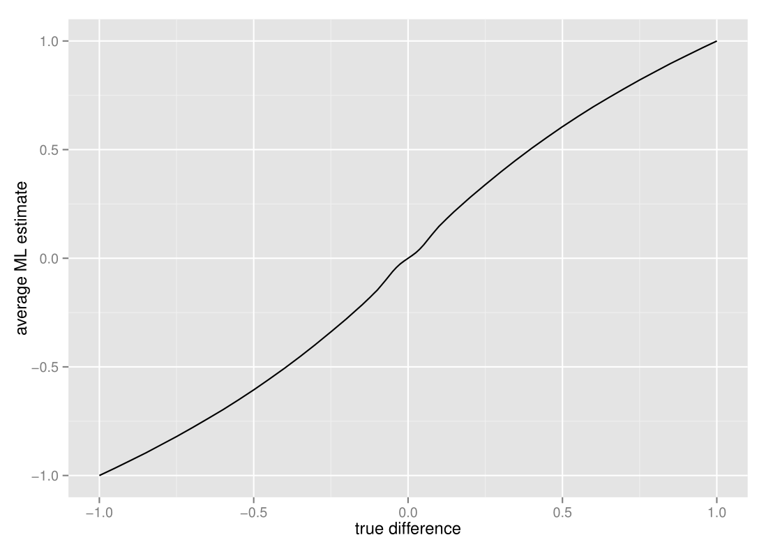
It seems like the average estimate is slightly off - to get a better view, let’s take a look at just the bias, i.e. the average ML estimate minus the true difference :
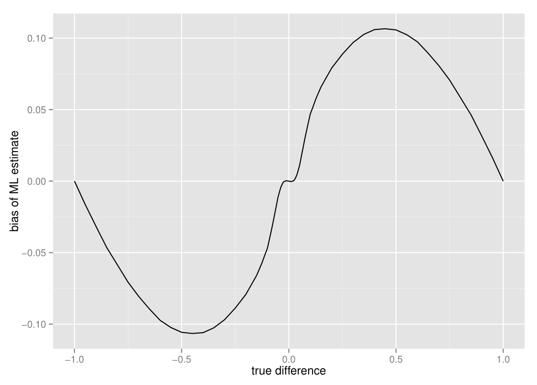
The estimates are (almost imperceptably) biased inwards when the true difference is close to zero, biased outwards when the difference between proportions are relatively large, and then unbiased again at the extreme ends. This is quite unlike fixed sample-size tests, which have no such bias at all. The reason for this difference is that there is an interaction between the stopping time and the estimate - sequential tests stop early when our samples are more extreme than some threshold, which means that the final estimates we get more often than not will be more extreme than what is true.
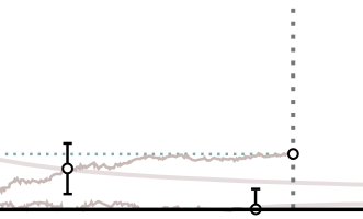
This might become a bit more intuitive if we take a look at a typical sample path for the MLE and the approximate thresholds for stopping the test in terms of the MLE. In this case the true difference is 0.2, and we do a two-sided sequential GLR test with α-level 0.05, β-level 0.10 and indifference region of size 0.1 :
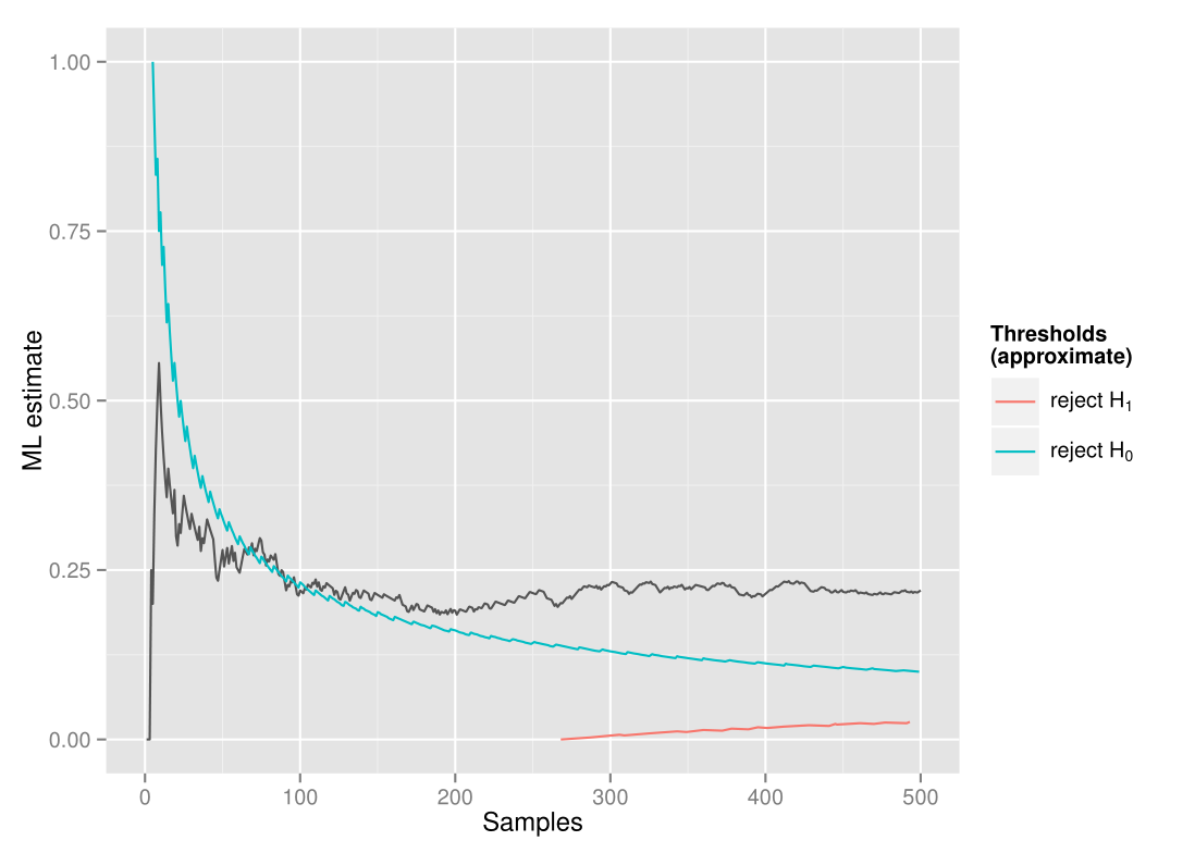
As we collect data, the ML estimates jump quite a bit around before converging towards the true difference. As it jumps around, it's likely to cross the threshold at a higher point (as seen happening here after around 70 samples) and thus stop the test at this point. Similarly, when the true difference is close to zero, it will usually stop at values slightly closer to zero than the actual difference. What about the vanishing bias at the extremes? This is because at the most extreme values, the test will almost invariably stop at only a handful of samples, and thus the interaction between the stopping time and the estimate practically disappears.
So what can we do about this problem? Unfortunately, there is not an uniformly best estimator we can use as a replacement for the MLE. Some of the estimators suggested to fix the bias have much larger mean squared error than the MLE due to having larger variance. However, a simple and commonly used correction (and what we use in the sequential A/B-testing library SeGLiR), is the Whitehead bias-adjusted estimate. The Whitehead bias-adjusted estimate is based on the fact that we know that:
E(\hat{\theta}) = \theta + b(\theta)
where theta is the true difference, theta_hat is our estimate of the difference, and b(theta) is the bias of our test at theta. Given an estimate theta_hat, we can then find an approximately bias-adjusted estimate by solving for theta_sim so that:
\tilde{\theta} + b(\tilde{\theta}) = \hat{\theta}
This can be found by simple simulation and some optimization. Note that there are also other alternative estimators, such as the conditional MLE, but since the brute-force simulation approach to this would take much more time than the Whitehead bias-adjustment, it's not something I've implemented in SeGLiR currently.
One important thing to note is that the bias problem is not specific to the sequential GLR test or even sequential frequentist tests. In fact any test with a stopping rule that depends on the parameter we estimate, such as Thompson sampling with a stopping rule (as used by google analytics) will have the same problem. John Kruschke discusses this in the context of bayesian analysis in this blog post.
Precision and Confidence intervals
So, given that we've bias-corrected the estimates, how precise are the estimates we get? Unfortunately, estimates from sequential analysis tests often are less precise than the fixed sample-size test. This is not so surprising, since the tests often stop earlier, and we thus have less data to base the estimates on. To see this for yourself, take a look at the estimates given in this demo.
For this reason, it is natural to ask for confidence intervals to bound the estimates in sequential analysis tests. Classical fixed sample-size tests use the normal approximation to create confidence intervals for the estimate. This is usually not possible with sequential analysis tests, since the distribution of the test statistics under a stopping rule are very complex and usually impossible to approximate by common distributions. Instead we can resort to bootstrap confidence intervals, which are simple to simulate. These are unfortunately also sensitive to the bias issues above, so the best option is to use a bias-adjusted confidence interval[1]. Note that since sequential tests stop early and we often have fewer samples, the confidence intervals will usually be wider than for the fixed sample-size test.
[1] see Davison & Hinkley : Bootstrap Methods and their applications, chap. 5.3 for details
P-values
As a little aside, what about p-values, the statistic everyone loves to hate?
When doing classical hypothesis tests, p-values are usually used to describe the significance of the result we find. This is not quite as good an idea in sequential tests as in fixed sample-size tests. The reason for this is that the p-value is not uniquely defined in sequential tests. The p-value is defined as the probability that we get a result as extreme or more extreme than the one we see, given that the null-hypothesis is true. In fixed sample-size tests, a more extreme result is simply a result where the test statistic is well, more extreme. However, in the sequential setting, we also have the variable of when the test was stopped. So is a more “extreme result” then a test that stops earlier? Or a test that stops later, but with a more “extreme” test-statistic? There is no definite answer to this. In the statistical literature there are several different ways to “order” the outcomes and thus define what is more “extreme”, but unfortunately there is no consensus on which “ordering” is the best, which makes p-values in sequential analysis a somewhat ambiguous statistic.
Nevertheless, in SeGLiR we've implemented a p-value via simple simulation, where we assume that a more “extreme result” is any result where the test statistic is more extreme than our result, regardless of when the test was stopped. This is what is called a Likelihood Ratio-ordering and is the ordering suggested by Cook & DeMets in their book referenced below.
As we've seen in this post, estimation in sequential tests is a bit more tricky than in fixed sample-size tests. Because sequential tests use much less samples, estimates may be more imprecise, and because of the interaction with the stopping rule they tend to be biased, though there are ways to mitigate the worst effects of this. In an upcoming post, I'm planning to compare sequential analysis tests with other variants of A/B-tests such as multi-armed bandits, and give a little guide on when to choose which test. If you're interested, follow me on twitter for updates.
References
If you're interested in more details on estimation in sequential tests, here are some recommended books that cover this subject. While these are mostly about group sequential tests, the solutions are the same as in the case with fully sequential tests (which is what I've described in my posts).
- C. Jennison & B. Turnbull : Group Sequential Methods with Applications to Clinical Trials, CRC Press 1999
- T. Cook & D. DeMets : Introduction to Statistical Methods for Clinical Trials, Chapman & Hall/CRC Press 2007